Kalman Filtering: A Simple Introduction
If a dynamic system is linear and with Gaussian noise, the optimal estimator of the hidden states is the Kalman Filter.
Application Example
In the engineering world, Kalman filters are one of the most common models to reduce noise from sensor signals. As we will discover, these models are extremely powereful when the noise in the data is roughly Gaussian.
Although they are a powerful tool for noise reduction, Kalman filters can be used for much more, here is an example: Say we have a jet engine with a fatigue crack growing on one of its components. We are trying to monitor the crack length with a stress sensor on such component.
Let’s assume we have measurements of the crack at every instance. Let’s also assume the crack length grows linearly with stress ( In reality, according to the Paris Law, it’s actually the log of the crack growth rate that grows linearly with the log of the stress intensity factor).
Kalman filters involve the following variables:
- Z: The observed variable (what we are trying to predict)
- X: The hidden state variable (what we use to predict Z, and ideally has a linear relationship with Z)
In our example, the observed variable is the crack length. Our hidden state variable is stress. Since we assumed there is a linear relationship between the two, and if we assume the noise is Gaussian, the optimal estimator is the Kalman Filter!
The Kalman Filter
The Kalman filter is an online learning algorithm. The model updates its estimation of the weights sequentially as new data comes in. Keep track of the notation of the subscripts in the equations. The current time step is denoted as n (the timestep for which we want to make a prediction).
PREVIOUS STATES
The ultimate goal of the Kalman filter is to predict the next observation of the observed variable Z by taking the best estimation of the hidden state variable X. One can then predict the next observation of Z by reconstructing it using X.
| The estimate of the observed variable Z is given by a linear transform H of the hidden states X. The subscript n represents the current timestep. Xn | n-1 represents the estimate of the hidden state X at timestep n given the data up to n-1. |
From this estimate of Z at timestep n, we can formulate the innovation:
The innovation Y is the difference between the prediction of the next observed state and the real observation of the next state.
To estimate the hidden state X, the Kalman Filter assumes that the transition from the hidden state to the observed variable has Gaussian noise. In the jet engine example, the measurement device may add noise to the system with inaccurate measurements of the crack length. These errors are assumed to be gaussian.
So every time a new observation comes in, the model estimates the hidden states X, and also carries forward an estimation of the uncertainty P. Together they parametrize a probability density function of the estimate of the observed variable. The predicted observation for the next time step will be the maximum likelihood estimate (the mean).
The first equation shows the estimate of the hidden state given the previous hidden state. F is the transition function from the previous state estimation to the current state estimation.
The second equation is the updated estimation of the uncertainty P. This is the covariance matrix, and it is a function of the covariance matrix of the previous state.
STATE UPDATE EQUATIONS
| So far, we have formulated the states given the data up to the previous time step (STATE n | n-1). We want to formulate an update for the new states given the new datapoint we have received at time step n, (STATE n | n). |
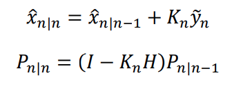
By minimizing the mean squared error, one can derive the optimal update of the hidden states X and the covariance P for timestep n.
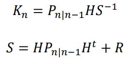
Where:
The first equation is the update of the hidden state n given all the data. The updated X is given by the previous estimation of the weights plus a gain term times the innovation. This is the same structure of the update found in the Recursive Least Squares (RLS) online learning algorithm.
The Kalman gain K at a timestep n is given by the previous estimation of the uncertainty P, the linear function H, and the inverse of the innovation covariance S.
With these equations, we can now implement our own Kalman Filter.
Example Implementation
A simple auto-regressive time series data will be used. The Kalman filter will be implemented and used to estimate the hidden states X, and then predict the next observations of Z.
The order of the autoregressive time series seen above will be set to 2. v(n) represents the white noise added to the system. With randomly initialized weights a, the autoregressive time series generates new points by multiplying the previous two points by the weights.
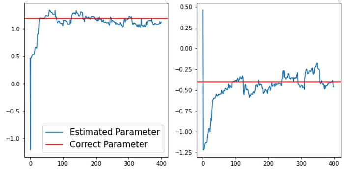
Above is the estimation of the hidden state X. The real value is shown in red, the Kalman estimation is shown in blue. As you can see the model is quick to converge to the approximate value of the hidden state. The model never estimates it perfectly due to the Gaussian noise added to the signal.
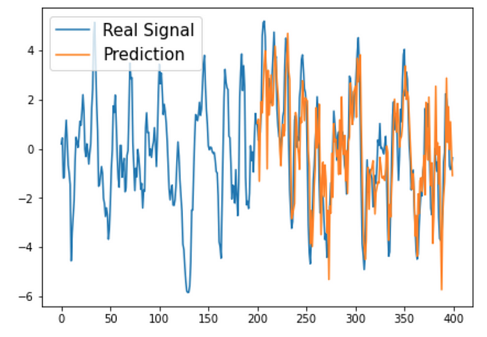
After around 200 observations, the model can accurately estimate the observed variable Z in the future. What is most impressive about Kalman filters and other online learning algorithms is their speed of convergence.
Where the Kalman Filter Fails
So far we have assumed the relationship between the hidden state and the observed state is linear, and we saw the model worked quite well. But what happens when we change this relationship to a nonlinear one.
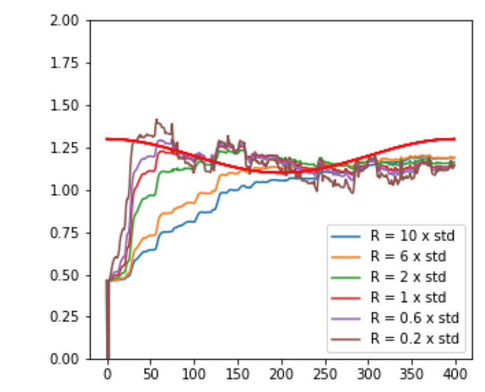
These are the estimations of the Kalman filter of one of the hidden states X that is changing over time in a sinusoidal wave. The model fails to generate good estimations of the hidden state X. Moreover, the predictions seem to lag behind the real values.
There are two hyperparameters I did not mention in the equations seen earlier. Q is the process noise covariance, and R is the measurement noise variance. By tuning R, we can make the model adapt quicker to changes in the hidden state. Adapting Q allows controlling how sensitive the model will be to process noise.
Even after tuning these hyperparameters, you can see the model lags behind the change in the hidden state variable, making its predictions less good. The Kalman filter is the optimal algorithm for linear systems, but when there is a non-linear relationship between the hidden state variable and the observed variable, these models tend to underperform.
Conclusion
The Kalman filter is extremely powerful and is used in a wide variety of fields, particularly in signal processing in engineering applications.
In a previous article, I described one of the simplest online learning algorithm, the Recursive Least Squares (RLS) algorithm. The Kalman Filter takes the RLS algorithm a step further, it assumes that there is Gaussian noise in the system. When predicting, the Kalman filter estimates the mean and covariance of the hidden state. The algorithm is essentially constructing a distribution around the predicted point, with the mean being the maximum likelihood estimation.


