Paper note - [Week 5]

Paper note - [Week 5]

A COMPREHENSIVE REVIEW OF YOLO ARCHITECTURES IN COMPUTER VISION: FROM YOLOV1 TO YOLOV8 AND YOLO-NAS

1. Object Detection Metrics and Non-Maximum Suppression (NMS)

The Average Precision (AP), traditionally called Mean Average Precision (mAP), is the commonly used metric for evaluating the performance of object detection models. It measures the average precision across all categories, providing a single value to compare different models. The COCO dataset makes no distinction between AP and mAP. In the rest of this paper, we will refer to this metric as AP.

1.1. How AP works?

The AP metric is based on precision-recall metrics, handling multiple object categories, and defining a positive prediction using Intersection over Union (IoU).

• Precision and Recall: Precision measures the accuracy of the model’s positive predictions, while recall measures the proportion of actual positive cases that the model correctly identifies. There is often a trade-off between precision and recall; for example, increasing the number of detected objects (higher recall) can result in more false positives (lower precision). To account for this trade-off, the AP metric incorporates the precision-recall curve that plots precision against recall for different confidence thresholds. This metric provides a balanced assessment of precision and recall by considering the area under the precision-recall curve.

• Handling multiple object categories: Object detection models must identify and localize multiple object categories in an image. The AP metric addresses this by calculating each category’s average precision (AP) separately and then taking the mean of these APs across all categories (that is why it is also called mean average precision). This approach ensures that the model’s performance is evaluated for each category individually, providing a more comprehensive assessment of the model’s overall performance.

• Intersection over Union: Object detection aims to accurately localize objects in images by predicting bounding boxes. The AP metric incorporates the Intersection over Union (IoU) measure to assess the quality of the predicted bounding boxes. IoU is the ratio of the intersection area to the union area of the predicted bounding box and the ground truth bounding box. It measures the overlap between the ground truth and predicted bounding boxes. The COCO benchmark considers multiple IoU thresholds to evaluate the model’s performance at different levels of localization accuracy.

1.2. Computing AP

a. VOC Dataset

This dataset includes 20 object categories. To compute the AP in VOC, we follow the next steps:

• For each category, calculate the precision-recall curve by varying the confidence threshold of the model’s predictions.
• Calculate each category’s average precision (AP) using an interpolated 11-point sampling of the precision-recall curve.
• Compute the final average precision (AP) by taking the mean of the APs across all 20 categories.

b. Microsoft COCO Dataset

This dataset includes 80 object categories and uses a more complex method for calculating AP. Instead of using an 11-point interpolation, it uses a 101-point interpolation, i.e., it computes the precision for 101 recall thresholds from 0 to 1 in increments of 0.01. Also, the AP is obtained by averaging over multiple IoU values instead of just one, except for a common AP metric called $AP_{50}$, which is the AP for a single IoU threshold of 0.5. The steps for computing AP in COCO are the following:

• For each category, calculate the precision-recall curve by varying the confidence threshold of the model’s predictions.
• Compute each category’s average precision (AP) using 101-recall thresholds.
• Calculate AP at different Intersection over Union (IoU) thresholds, typically from 0.5 to 0.95 with a step size of 0.05. A higher IoU threshold requires a more accurate prediction to be considered a true positive.
• For each IoU threshold, take the mean of the APs across all 80 categories.
• Finally, compute the overall AP by averaging the AP values calculated at each IoU threshold.

The differences in AP calculation make it hard to directly compare the performance of object detection models across the two datasets. The current standard uses the COCO AP due to its more fine-grained evaluation of how well a model performs at different IoU thresholds.

1.3. Non-Maximum Suppression (NMS)

Non-Maximum Suppression (NMS) is a post-processing technique used in object detection algorithms to reduce the number of overlapping bounding boxes and improve the overall detection quality. Object detection algorithms typically generate multiple bounding boxes around the same object with different confidence scores. NMS filters out redundant and irrelevant bounding boxes, keeping only the most accurate ones. Algorithm 1 describes the procedure. Figure 4 shows the typical output of an object detection model containing multiple overlapping bounding boxes and the output after NMS.

2. YOLO: You Only Look Once (CVPR 2016)

YOLO by Joseph Redmon et al. was published in CVPR 2016. It presented for the first time a real-time end-to-end approach for object detection. The name YOLO stands for “You Only Look Once,” referring to the fact that it was able to accomplish the detection task with a single pass of the network, as opposed to previous approaches that either used sliding windows followed by a classifier that needed to run hundreds or thousands of times per image or the more advanced methods that divided the task into two-steps, where the first step detects possible regions with objects or regions proposals and the second step run a classifier on the proposals. Also, YOLO used a more straightforward output based only on regression to predict the detection outputs as opposed to Fast R-CNN that used two separate outputs, a classification for the probabilities and a regression for the boxes coordinates.

YOLOv1 unified the object detection steps by detecting all the bounding boxes simultaneously.

To accomplish this, YOLO divides the input image into a $S × S$ grid and predicts $B$ bounding boxes of the same class, along with its confidence for $C$ different classes per grid element. Each bounding box prediction consists of five values: $P_c, b_x, b_y, b_h, b_w$ where $P_c$ is the confidence score for the box that reflects how confident the model is that the box contains an object and how accurate the box is. The $b_x$ and $b_y$ coordinates are the centers of the box relative to the grid cell, and $b_h$ and $b_w$ are the height and width of the box relative to the full image. The output of YOLO is a tensor of $S × S × (B × 5 + C)$ optionally followed by non-maximum suppression (NMS) to remove duplicate detections.

In the original YOLO paper, the authors used the PASCAL VOC dataset that contains 20 classes (C = 20); a grid of 7 × 7 (S = 7) and at most 2 classes per grid element (B = 2), giving a 7 × 7 × 30 output prediction.

YOLOv1 Architecture

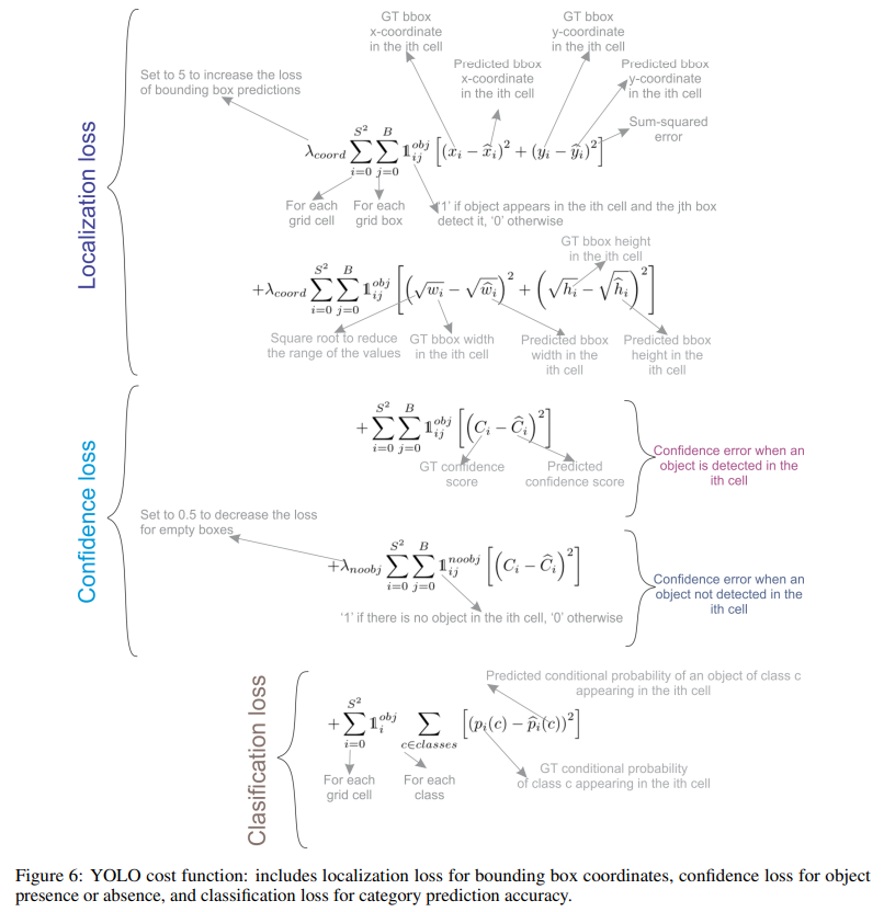
Loss function

YOLOv1 Strengths and Limitations

Strengths:

The simple architecture of YOLO, along with its novel full-image one-shot regression, made it much faster than the existing object detectors allowing real-time performance.

Limitation:

• It could only detect at most two objects of the same class in the grid cell, limiting its ability to predict nearby objects.

• It struggled to predict objects with aspect ratios not seen in the training data.

• It learned from coarse object features due to the down-sampling layers.

3. YOLOv2: Better, Faster, and Stronger (CVPR 2017)

Improvements

• Batch normalization on all convolutional layers improved convergence and acts as a regularizer to reduce overfitting.

• High-resolution classifier: Like YOLOv1, they pre-trained the model with ImageNet at 224 × 224. However, this time, they finetuned the model for ten epochs on ImageNet with a resolution of 448 × 448, improving the network performance on higher resolution input.

• Fully convolutional: They removed the dense layers and used a fully convolutional architecture.

• Use anchor boxes to predict bounding boxes: They use a set of prior boxes or anchor boxes, which are boxes with predefined shapes used to match prototypical shapes of objects as shown in Figure below. Multiple anchor boxes are defined for each grid cell, and the system predicts the coordinates and the class for every anchor box. The size of the network output is proportional to the number of anchor boxes per grid cell.

• Dimension Clusters: Picking good prior boxes helps the network learn to predict more accurate bounding boxes. The authors ran k-means clustering on the training bounding boxes to find good priors. They selected five prior boxes providing a good tradeoff between recall and model complexity.

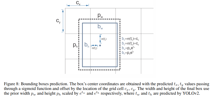
• Direct location prediction: Unlike other methods that predicted offsets, YOLOv2 followed the same philosophy and predicted location coordinates relative to the grid cell. The network predicts five bounding boxes for each cell, each with five values $t_x, t_y, t_w, t_h$, and $t_o$, where to is equivalent to $P_c$ from YOLOv1 and the final bounding box coordinates are obtained.

• Finner-grained features: YOLOv2, compared with YOLOv1, removed one pooling layer to obtain an output feature map or grid of 13 × 13 for input images of 416 × 416. YOLOv2 also uses a passthrough layer that takes the 26 × 26 × 512 feature map and reorganizes it by stacking adjacent features into different channels instead of losing them via a spatial subsampling. This generates 13 × 13 × 2048 feature maps concatenated in the channel dimension with the lower resolution 13 × 13 × 1024 maps to obtain 13 × 13 × 3072 feature maps.

• Multi-scale training: Since YOLOv2 does not use fully connected layers, the inputs can be different sizes. To make YOLOv2 robust to different input sizes, the authors trained the model randomly, changing the input size —from 320 × 320 up to 608 × 608— every ten batches.

YOLOv2 Architecture (Darknet-19)

4. YOLOv3 (ArXiv 2018)

Improvements

• Bounding box prediction: Like YOLOv2, the network predicts four coordinates for each bounding box $t_x, t_y, t_w$, and $t_h$; however, this time, YOLOv3 predicts an objectness score for each bounding box using logistic regression. This score is 1 for the anchor box with the highest overlap with the ground truth and 0 for the rest anchor boxes. YOLOv3, as opposed to Faster R-CNN, assigns only one anchor box to each ground truth object. Also, if no anchor box is assigned to an object, it only incurs in classification loss but not localization loss or confidence loss.

• Class Prediction: Instead of using a softmax for the classification, they used binary cross-entropy to train independent logistic classifiers and pose the problem as a multilabel classification. This change allows assigning multiple labels to the same box, which may occur on some complex datasets with overlapping labels. For example, the same object can be a Person and a Man.

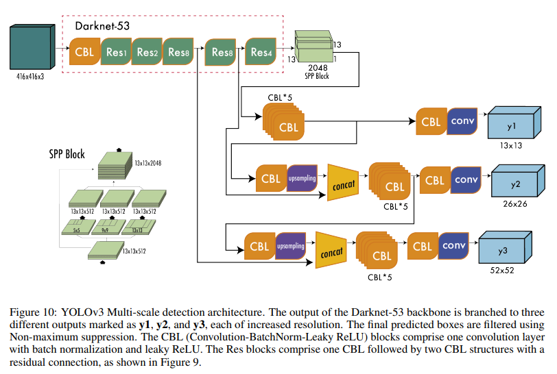
• New backbone: YOLOv3 features a larger feature extractor composed of 53 convolutional layers with residual connections.

• Spatial pyramid pooling (SPP): Although not mentioned in the paper, the authors also added to the backbone a modified SPP block that concatenates multiple max pooling outputs without subsampling (stride = 1), each with different kernel sizes k × k where k = 1, 5, 9, 13 allowing a larger receptive field. This version is called YOLOv3-spp and was the best-performed version improving the $AP_{50}$ by 2.7%.

• Multi-scale Predictions; Similar to Feature Pyramid Networks, YOLOv3 predicts three boxes at three different scales.

• Bounding box priors: Like YOLOv2, the authors also use k-means to determine the bounding box priors of anchor boxes. The difference is that in YOLOv2, they used a total of five prior boxes per cell, and in YOLOv3, they used three prior boxes for three different scales.

YOLOv3 Architecture

Note:

• The backbone is responsible for extracting useful features from the input image. It is typically a convolutional neural network (CNN) trained on a large-scale image classification task, such as ImageNet. The backbone captures hierarchical features at different scales, with lower-level features (e.g., edges and textures) extracted in the earlier layers and higher-level features (e.g., object parts and semantic information) extracted in the deeper layers.

• The neck is an intermediate component that connects the backbone to the head. It aggregates and refines the features extracted by the backbone, often focusing on enhancing the spatial and semantic information across different scales. The neck may include additional convolutional layers, feature pyramid networks (FPN), or other mechanisms to improve the representation of the features.

• The head is the final component of an object detector; it is responsible for making predictions based on the features provided by the backbone and neck. It typically consists of one or more task-specific subnetworks that perform classification, localization, and, more recently, instance segmentation and pose estimation. The head processes the features the neck provides, generating predictions for each object candidate. In the end, a post-processing step, such as non-maximum suppression (NMS), filters out overlapping predictions and retains only the most confident detections.

5. YOLOv4 (ArViv 2020)

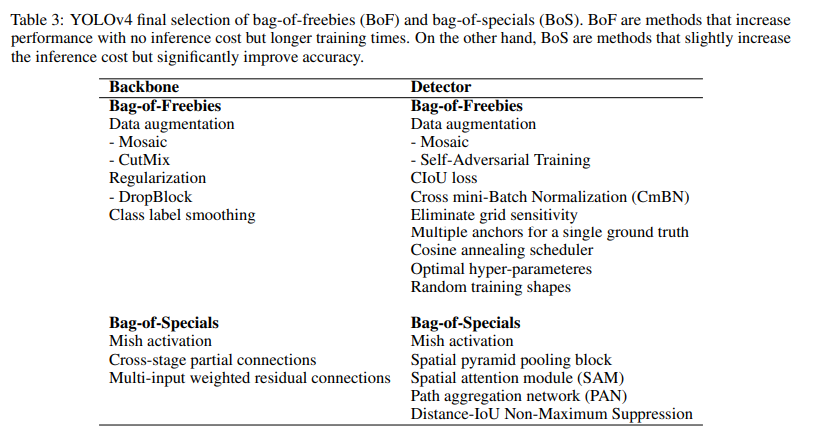
YOLOv4 tried to find the optimal balance by experimenting with many changes categorized as bag-of-freebies and bag-of-specials. Bag-of-freebies are methods that only change the training strategy and increase training cost but do not increase the inference time, the most common being data augmentation. On the other hand, bag-of-specials are methods that slightly increase the inference cost but significantly improve accuracy. Examples of these methods are those for enlarging the receptive field, combining features, and post-processing among others.

Improvements

• An Enhanced Architecture with Bag-of-Specials (BoS) Integration

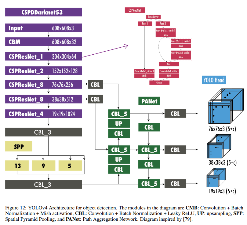
The authors tried multiple architectures for the backbone, such as ResNeXt50, EfficientNet-B3, and Darknet-53. The best-performing architecture was a modification of Darknet-53 with cross-stage partial connections (CSPNet), and Mish activation function as the backbone. For the neck, they used the modified version of spatial pyramid pooling (SPP) from YOLOv3-spp and multi-scale predictions as in YOLOv3, but with a modified version of path aggregation network (PANet) instead of FPN as well as a modified spatial attention module (SAM). Finally, for the detection head, they use anchors as in YOLOv3. Therefore, the model was called CSPDarknet53-PANet-SPP. The cross-stage partial connections (CSP) added to the Darknet-53 help reduce the computation of the model while keeping the same accuracy. The SPP block, as in YOLOv3-spp increases the receptive field without affecting the inference speed. The modified version of PANet concatenates the features instead of adding them as in the original PANet paper.

• Integrating bag-of-freebies (BoF) for an Advanced Training Approach

Apart from the regular augmentations such as random brightness, contrast, scaling, cropping, flipping, and rotation, the authors implemented mosaic augmentation that combines four images into a single one allowing the detection of objects outside their usual context and also reducing the need for a large mini-batch size for batch normalization. For regularization, they used DropBlock that works as a replacement of Dropout but for convolutional neural networks as well as class label smoothing. For the detector, they added CIoU loss and Cross mini-bath normalization (CmBN) for collecting statistics from the entire batch instead of from single mini-batches as in regular batch normalization.

• Self-adversarial Training (SAT)

To make the model more robust to perturbations, an adversarial attack is performed on the input image to create a deception that the ground truth object is not in the image but keeps the original label to detect the correct object.

• Hyperparameter Optimization with Genetic Algorithms

To find the optimal hyperparameters used for training, they use genetic algorithms on the first 10% of periods, and a cosine annealing scheduler to alter the learning rate during training. It starts reducing the learning rate slowly, followed by a quick reduction halfway through the training process ending with a slight reduction.

YOLOv4 Architecture

6. YOLOv5 (Ultralytics 2020)

Improvements

• Developed in Pytorch instead of Darknet.

• YOLOv5 incorporates an Ultralytics algorithm called AutoAnchor. This pre-training tool checks and adjusts anchor boxes if they are ill-fitted for the dataset and training settings, such as image size. It first applies a k-means function to dataset labels to generate initial conditions for a Genetic Evolution (GE) algorithm. The GE algorithm then evolves these anchors over 1000 generations by default, using CIoU loss and Best Possible Recall as its fitness function.

YOLOv5 Architecture

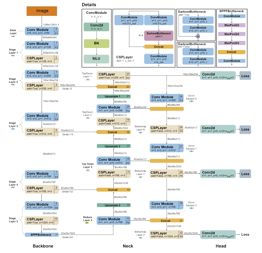
YOLOv5 Architecture. The architecture uses a modified CSPDarknet53 backbone with a Stem, followed by convolutional layers that extract image features. A spatial pyramid pooling fast (SPPF) layer accelerates computation by pooling features into a fixed-size map. Each convolution has batch normalization and SiLU activation. The network’s neck uses SPPF and a modified CSP-PAN, while the head resembles YOLOv3.

7. Scaled-YOLOv4 and YOLOR

7.1. Scaled-YOLOv4 (CVPR 2021)

Differently from YOLOv4, Scaled YOLOv4 was developed in Pytorch instead of Darknet. The main novelty was the introduction of scaling-up and scaling-down techniques. Scaling up means producing a model that increases accuracy at the expense of a lower speed; on the other hand, scaling down entails producing a model that increases speed sacrificing accuracy. In addition, scaled-down models need less computing power and can run on embedded systems.

7.2. YOLOR (ArXiv 2021)

It stands for You Only Learn One Representation. In this paper, the authors followed a different approach; they developed a multi-task learning approach that aims to create a single model for various tasks (e.g., classification, detection, pose estimation) by learning a general representation and using sub-networks to create task-specific representations. With the insight that the traditional joint learning method often leads to suboptimal feature generation, YOLOR aims to overcome this by encoding the implicit knowledge of neural networks to be applied to multiple tasks, similar to how humans use past experiences to approach new problems. The results showed that introducing implicit knowledge into the neural network benefits all the tasks.

8. YOLOX (ArXiv 2021)

Main changes of YOLOX with respect to YOLOv3.

Improvements

• Anchor-free: Since YOLOv2, all subsequent YOLO versions were anchor-based detectors. YOLOX, inspired by anchor-free state-of-the-art object detectors such as CornerNet, CenterNet, and FCOS, returned to an anchor-free architecture simplifying the training and decoding process. The anchor-free increased the AP by 0.9 points concerning the YOLOv3 baseline.

• Multi positives: To compensate for the large imbalances the lack of anchors produced, the authors use center sampling where they assigned the center 3 × 3 area as positives. This approach increased AP by 2.1 points.

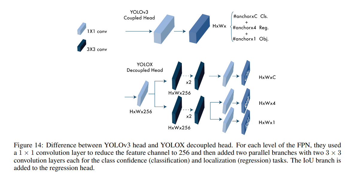
• Decoupled head: YOLOX separates these two into two heads, one for classification tasks and the other for regression tasks improving the AP by 1.1 points and speeding up the model convergence.

• Advanced label assignment: Proposed a simplified version called simOTA. This change increased AP by 2.3 points.

• Strong augmentations: YOLOX uses MixUP and Mosaic augmentations. The authors found that ImageNet pretraining was no longer beneficial after using these augmentations. The strong augmentations increased AP by 2.4 points.

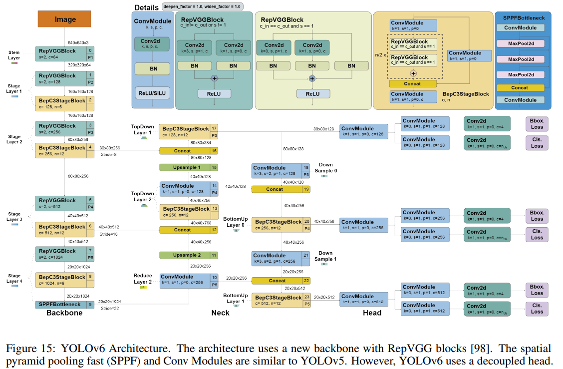
9. YOLOv6 (ArXiv 2022)

Improvements

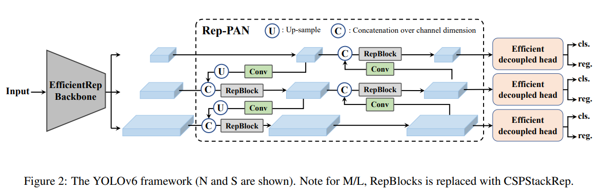
• A new backbone based on RepVGG: called EfficientRep that uses higher parallelism than previous YOLO backbones. For the neck, they use PAN enhanced with RepBlocks or CSPStackRep Blocks for the larger models. And following YOLOX, they developed an efficient decoupled head.

• Label assignment using the Task alignment learning approach introduced in TOOD.

• New classification and regression losses: They used a classification VariFocal loss and an SIoU/GIoU regression loss.

• A self-distillation strategy for the regression and classification tasks.

• A quantization scheme for detection using RepOptimizer and channel-wise distillation that helped to achieve a faster detector.

YOLOv6 Architecture

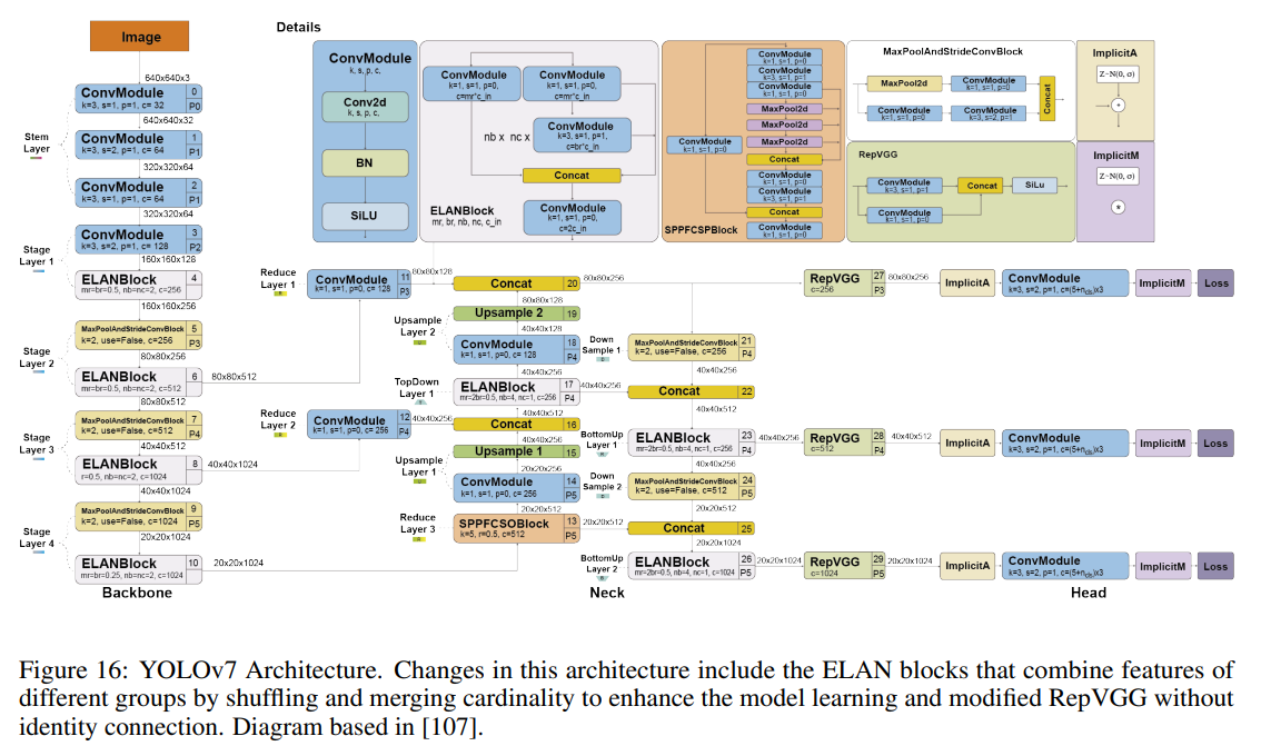
10. YOLOv7 (ArXiv 2022)

Improvements

The architecture changes of YOLOv7 are:

• Extended efficient layer aggregation network (E-ELAN): ELAN is a strategy that allows a deep model to learn and converge more efficiently by controlling the shortest longest gradient path. YOLOv7 proposed E-ELAN that works for models with unlimited stacked computational blocks. E-ELAN combines the features of different groups by shuffling and merging cardinality to enhance the network’s learning without destroying the original gradient path.

• Model scaling for concatenation-based models: Scaling generates models of different sizes by adjusting some model attributes. The architecture of YOLOv7 is a concatenation-based architecture in which standard scaling techniques, such as depth scaling, cause a ratio change between the input channel and the output channel of a transition layer which, in turn, leads to a decrease in the hardware usage of the model. YOLOv7 proposed a new strategy for scaling concatenation-based models in which the depth and width of the block are scaled with the same factor to maintain the optimal structure of the model.

The bag-of-freebies used in YOLOv7 include:

• Planned re-parameterized convolution: Like YOLOv6, the architecture of YOLOv7 is also inspired by re-parameterized convolutions (RepConv). However, they found that the identity connection in RepConv destroys the residual in ResNet and the concatenation in DenseNet. For this reason, they removed the identity connection and called it RepConvN.

• Coarse label assignment for auxiliary head and fine label assignment for the lead head. The lead head is responsible for the final output, while the auxiliary head assists with the training.

• Batch normalization in conv-bn-activation. This integrates the mean and variance of batch normalization into the bias and weight of the convolutional layer at the inference stage.

• Implicit knowledge inspired in YOLOR.

• Exponential moving average as the final inference model.

YOLOv7 Architecture

11. DAMO-YOLO (ArXiv 2022)

Improvements

• A Neural architecture search (NAS). They used a method called MAE-NAS [111] developed by Alibaba to find an efficient architecture automatically.

• A large neck. Inspired by GiraffeDet, CSPNet, and ELAN, the authors designed a neck that can work in real-time called Efficient-RepGFPN.

• A small head. The authors found that a large neck and a small neck yield better performance, and they only left one linear layer for classification and one for regression. They called this approach ZeroHead.

• AlignedOTA label assignment. Dynamic label assignment methods, such as OTA and TOOD, have gained popularity due to their significant improvements over static methods. However, the misalignment between classification and regression remains a problem, partly because of the imbalance between classification and regression losses. To address this issue, their AlignOTA method introduces focal loss into the classification cost and uses the IoU of prediction and ground truth box as the soft label, enabling the selection of aligned samples for each target and solving the problem from a global perspective.

• Knowledge distillation. Their proposed strategy consists of two stages: the teacher guiding the student in the first stage and the student fine-tuning independently in the second stage. Additionally, they incorporate two enhancements in the distillation approach: the Align Module, which adapts student features to the same resolution as the teacher’s, and Channel-wise Dynamic Temperature, which normalizes teacher and student features to reduce the impact of real value differences.

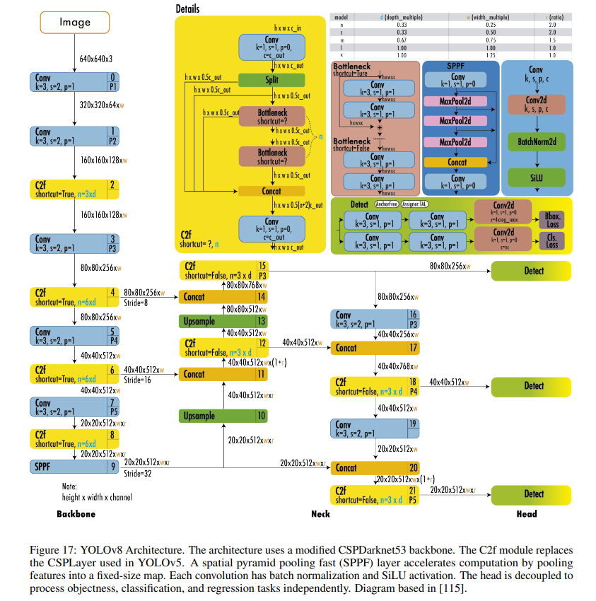
12. YOLOv8 (Ultralytics 2023)

Improvements

• YOLOv8 uses a similar backbone as YOLOv5 with some changes on the CSPLayer, now called the C2f module. The C2f module (cross-stage partial bottleneck with two convolutions) combines high-level features with contextual information to improve detection accuracy.

• YOLOv8 uses an anchor-free model with a decoupled head to independently process objectness, classification, and regression tasks. This design allows each branch to focus on its task and improves the model’s overall accuracy. In the output layer of YOLOv8, they used the sigmoid function as the activation function for the objectness score, representing the probability that the bounding box contains an object. It uses the softmax function for the class probabilities, representing the objects’ probabilities belonging to each possible class.

• YOLOv8 uses CIoU and DFL loss functions for bounding box loss and binary cross-entropy for classification loss. These losses have improved object detection performance, particularly when dealing with smaller objects.

• YOLOv8 also provides a semantic segmentation model called YOLOv8-Seg model. The backbone is a CSPDarknet53 feature extractor, followed by a C2f module instead of the traditional YOLO neck architecture. The C2f module is followed by two segmentation heads, which learn to predict the semantic segmentation masks for the input image. The model has similar detection heads to YOLOv8, consisting of five detection modules and a prediction layer. The YOLOv8-Seg model has achieved state-of-the-art results on various object detection and semantic segmentation benchmarks while maintaining high speed and efficiency.

YOLOv8 Architecture

13. PP-YOLO, PP-YOLOv2, and PP-YOLOE (PaddlePaddle based - ArXiv 2020)

… Nothing

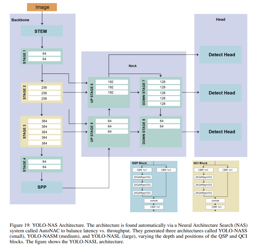
14. YOLO-NAS (2023)

YOLO-NAS is designed to detect small objects, improve localization accuracy, and enhance the performance-per-compute ratio, making it suitable for real-time edge-device applications. In addition, its open-source architecture is available for research use.

Improvements

• Quantization aware modules called QSP and QCI that combine re-parameterization for 8-bit quantization to minimize the accuracy loss during post-training quantization.

• Automatic architecture design using AutoNAC, Deci’s proprietary NAS technology.

• Hybrid quantization method to selectively quantize certain parts of a model to balance latency and accuracy instead of standard quantization, where all the layers are affected.

• A pre-training regimen with automatically labeled data, self-distillation, and large datasets.

15. YOLO with Transformers

15.1. YOLOS (NeurIPS 2021)

15.2. ViT-YOLO (ICCVW 2021)

15.3. MSFT-YOLO (MDPI Sensors 2022)

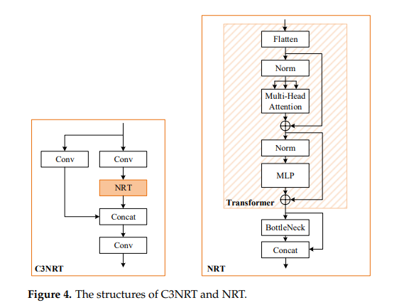
15.4. NRT-YOLO (MDPI Sensors 2022)

15.5. YOLO-SD (Remote Sensing 2022)

16. Summary

• Anchors: The original YOLO model was relatively simple and did not employ anchors, while the state-of-theart relied on two-stage detectors with anchors. YOLOv2 incorporated anchors, leading to improvements in bounding box prediction accuracy. This trend persisted for five years until YOLOX introduced an anchor-less approach that achieved state-of-the-art results. Since then, subsequent YOLO versions have abandoned the use of anchors.

• Framework: Initially, YOLO was developed using the Darknet framework, with subsequent versions following suit. However, when Ultralytics ported YOLOv3 to PyTorch, the remaining YOLO versions were developed using PyTorch, leading to a surge in enhancements. Another deep learning language utilized is PaddlePaddle, an open-source framework initially developed by Baidu.

• Backbone: The backbone architectures of YOLO models have undergone significant changes over time. Starting with the Darknet architecture, which comprised simple convolutional and max pooling layers, later models incorporated cross-stage partial connections (CSP) in YOLOv4, reparameterization in YOLOv6 and YOLOv7, and neural architecture search in DAMO-YOLO and YOLO-NAS.

• Performance: While the performance of YOLO models has improved over time, it is worth noting that they often prioritize balancing speed and accuracy rather than solely focusing on accuracy. This tradeoff is essential to the YOLO framework, allowing for real-time object detection across various applications.

YOLOv9: Learning What You Want to Learn Using Programmable Gradient Information

(ArXiv 2024)

Motivation

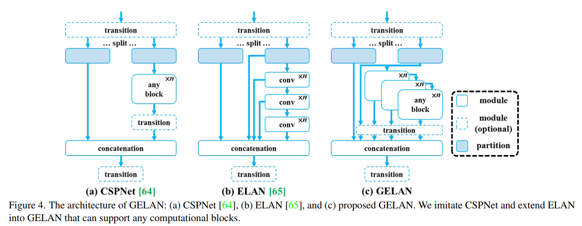
This paper introduces a novel concept named Programmable Gradient Information to address the issue of data loss in deep learning networks as data undergoes layer-by-layer feature extraction and spatial transformation. PGI aims to provide complete input information for calculating the objective function, ensuring reliable gradient information for network weight updates. Alongside PGI, the authors present a new lightweight network architecture called Generalized Efficient Layer Aggregation Network (GELAN), which is designed based on gradient path planning. GELAN leverages conventional convolution operators to achieve better parameter utilization compared to state-of-the-art methods that use depth-wise convolution. The effectiveness of GELAN and PGI is demonstrated through object detection tasks on the MS COCO dataset, showing that this approach allows train-from-scratch models to surpass the performance of models pre-trained on large datasets.

Contribution

• PGI - Programmable gradient information : Solves the problem that deep supervision can only be used for extremely deep neural network architectures, and therefore allows new lightweight architectures to be truly applied in daily life.

• GELAN - Generalized Efficient Layer Aggregation Networks : only uses conventional convolution to achieve a higher parameter usage than the depth-wise convolution design that based on the most advanced technology, while showing great advantages of being light, fast, and accurate.

Method

Problem Statement

Information Bottleneck Principle

The Information Bottleneck Principle highlights the inevitable information loss data X experiences during transformation in deep neural networks; it illustrates that with each layer the data passes through, the likelihood of information loss increases, potentially leading to unreliable gradients and poor network convergence due to incomplete information about the prediction target. One proposed solution to mitigate this issue is to enlarge the model with more parameters, allowing for a more comprehensive data transformation and improving the chances of retaining sufficient information for accurate target mapping. However, this approach does not address the fundamental issue of unreliable gradients in very deep networks. The authors suggest exploring reversible functions as a potential solution to maintain information integrity throughout the network, aiming to achieve better convergence by preserving essential data through the network layers.

Reversible Functions

The concept of reversible functions means that a function and its inverse can transform data without loss of information. This principle is applied in architectures like PreAct ResNet, which ensures data is passed through layers without loss, aiding in deep network convergence but potentially compromising the depth’s advantage in solving complex problems. An analysis using the information bottleneck principle reveals that retaining critical information mapping data to targets is essential for training effectiveness, especially in lightweight models. The aim is to develop a new training method that generates reliable gradients for model updates and is feasible for both shallow and lightweight neural networks, addressing the core issue of significant information loss during data transformation.

Approach

Programmable Gradient Information

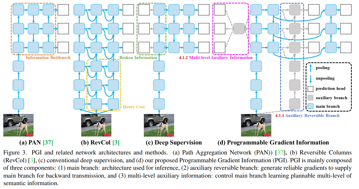
PGI consists of three components: a main branch for inference without extra cost, an auxiliary reversible branch to counteract the effects of network depth, and multi-level auxiliary information to mitigate error accumulation in deep supervision and lightweight models with multiple prediction branches.

Auxiliary Reversible Branch

Auxiliary Reversible Branch helps maintain complete information flow from data to targets, mitigating the risk of false correlations due to incomplete features. However, integrating a reversible architecture with a main branch significantly increases inference costs. To counteract this, PGI treats the reversible branch as an expansion of deep supervision, enhancing the main branch’s ability to capture relevant information without the necessity of retaining complete original data. This approach allows for effective parameter learning and application to shallower networks. Importantly, the auxiliary reversible branch can be omitted during inference, preserving the network’s original inference efficiency.

Multi-level Auxiliary Information

This component aims to address the information loss in deep supervision architectures, particularly in object detection tasks using multiple prediction branches and feature pyramids for detecting objects of various sizes. This component integrates a network between the feature pyramid layers and the main branch to merge gradient information from different prediction heads. This integration ensures that each feature pyramid receives comprehensive target object information, enabling the main branch to retain complete information for learning predictions across various targets. By aggregating gradient information containing data about all target objects, the main branch’s learning is not skewed towards specific object information, mitigating the issue of fragmented information in deep supervision.

Experiments

YOLOv9 outperforms existing real-time object detectors across various model sizes, achieving higher accuracy with fewer parameters and reduced computational requirements. Specifically, YOLOv9 surpasses lightweight and medium models like YOLO MS in terms of parameter efficiency and accuracy, matches the performance of general models such as YOLOv7 AF with significantly fewer parameters and calculations, and exceeds the large model YOLOv8-X in both efficiency and accuracy.

Additionally, when compared to models using depth-wise convolution or ImageNet pretraining, YOLOv9 demonstrates superior parameter utilization and computational efficiency. The success of YOLOv9, particularly in deep models, is attributed to the PGI, which enhances the ability to retain and extract crucial information for data-target mapping, leading to performance improvements while maintaining lower parameter and computation demands.

Ablations

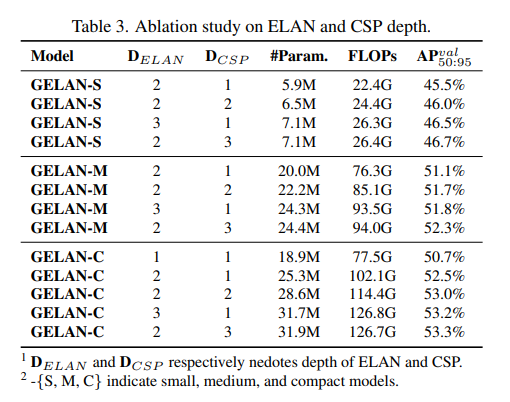
• CSP blocks were identified as particularly effective, enhancing performance with reduced parameters and improved accuracy, leading to their selection for GELAN in YOLOv9.

• GELAN’s performance is not highly sensitive to block depth, allowing for flexible architecture design without compromising stability.

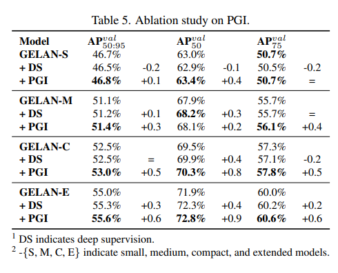
• Applying PGI’s auxiliary supervision to deep supervision concepts demonstrated significant improvements, particularly in deep models.