
Paper note - [Week 3]
Monocular 3D Vehicle Detection Using Uncalibrated Traffic Cameras through Homography
(IROS 2021)
Motivation
Traffic cameras are widely deployed today to monitor traffic conditions especially around intersections.
Monocular camera 3D object detection is a non-trivial task since images lack depth information.
Problem:
- The intrinsic/extrinsic calibration information of many cameras are not available to users.
- 3D annotations of images from these traffic cameras are lacking, while there are some with 2D annotations. (Some previous work tried to solve the 3D object detection problem, but they posed some strong assumptions such as known intrinsic/extrinsic calibration or fixed orientation of the objects)
Contribution
Propose a method to estimate the pose and position of vehicles in the 3D world using images from a monocular uncalibrated traffic camera.
Propose two strategies to improve the accuracy of object detection using IPM images: (a) tailed r-box regression, (b) dual-view network architecture.
Propose a data synthesis method to generate data that are visually similar to images from an uncalibrated traffic camera.
Method
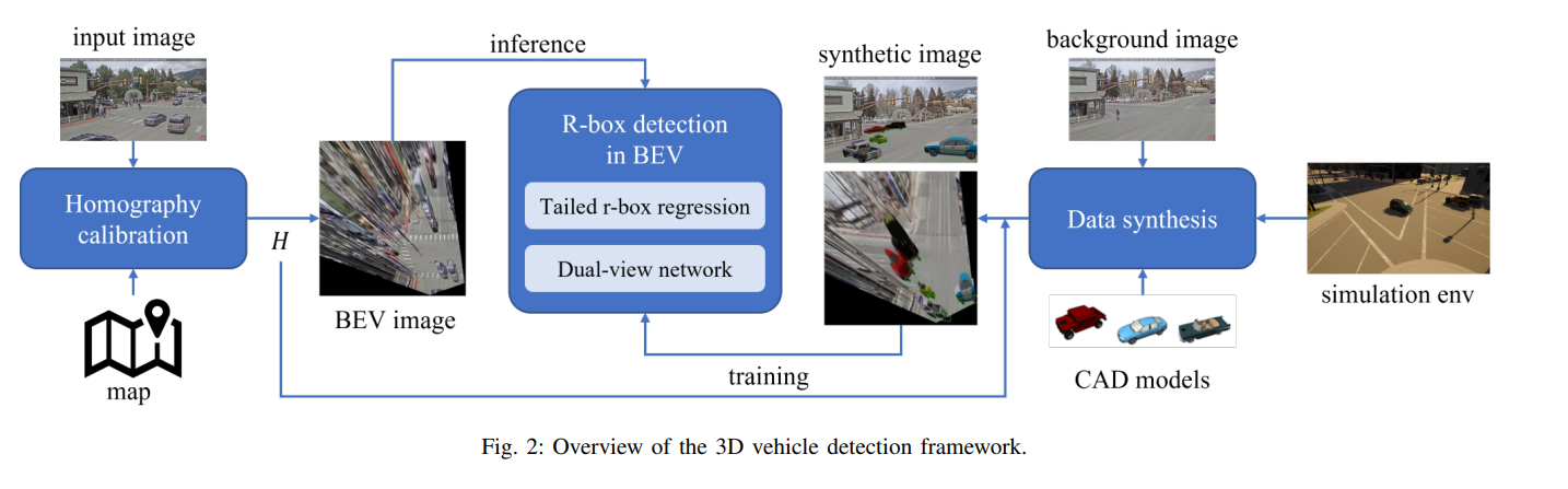
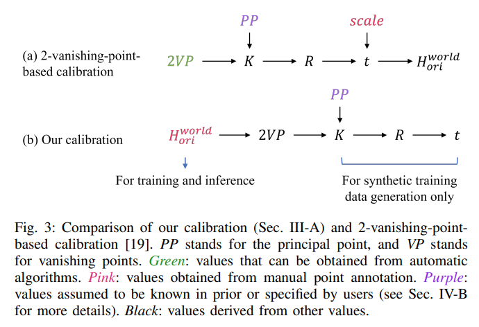
1. Calibration of homography
A planar homography is a mapping between two planes which preserves collinearity, represented by a 3*3 matrix. We model the homography between the original image and the bird’s eye view image as a composition of two homographies:
\[H^{bev}_{ori} = H^{bev}_{world} H^{world}_{ori}\]where $sp_a = H^a_b p_b$, denoting that $H^a_b$ maps coordinates in frame $b$ to coordinated in frame $a$ up to a scale factor $s$, and $p = [x, y, 1]^T$ is the homogeneous coordinate of a point in a plane.
bev denotes the BEV image plane.
world denotes the road plane in the real world.
ori denotes the original image plane.
$H^{bev}_{world}$ can be freely defined by users as long as it is a similarity transform, preserving the angles between the real-world road plane and the bird’s eye view image plane.
Calibration is needed for $H^{world}_{ori}$, denoting the homography between the original image plane and road plane in the real world.
=> Can be use if the intrinsic and extrinsic parameters of a camera is known.
In paper, they use satellite images for find corresponding points and use Direct Linear Transformation (DLT) to calculate $H^{world}_{ori}$.
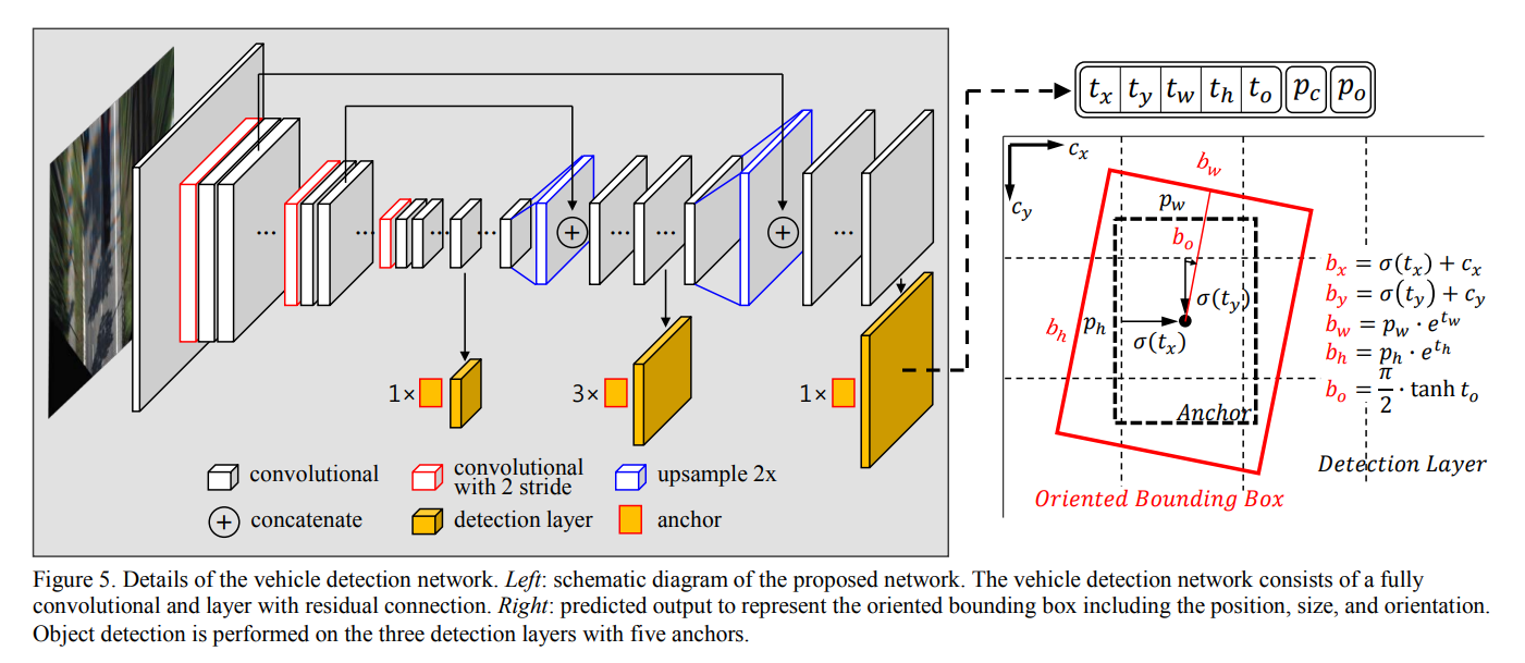
2. Rotated bounding box detection in warped bird’s eye view (BEV) images
The rotated bounding box detection network in this paper is developed based on YOLOv3, by extending it to support rotation prediction.
The network is extended to predict rotations by introducing the yaw ($r$) dimension in both anchors and predictions. The anchors are now of the form $(l, w, r)$, where $r ∈ [0, π]$, implying that we are not distinguishing the front end and rear end of vehicles in the network. Although the dimension of the anchors increased by one, we do not increase the total number of anchors, due to the fact that object size does not vary too much in our bird’s eye view images. There are 9 anchors per YOLO prediction layers, and there are in total 3 YOLO layers in the network, the same as in YOLOv3. The rotation angles of 9 anchors in a YOLO prediction layer are evenly distributed over the $[0, π]$ interval.
The network predicts the rotational angle offsets to the anchors. Denote the angle of an anchor as $r_0$, only anchors with $|r_0 − r_{gt}|< π/4$ can be considered as positive, and for a positive anchor the rotation angle is predicted following Eq. below.
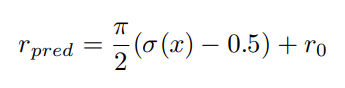
where $x$ is the output of a convolution layer, and $σ(·)$ is the sigmoid function. It follows that $|r_{pred} − r_0|< π/4$.
The loss function for angle prediction is in Eq. below. Note that the angular residual $r_{res} = r_{pred} − r_{gt} ∈ (−π/2, π/2)$ falls in a converging basin of the $sin^2(·)$ function.

3. Special designs for detection in warped BEV images
With the above setup, the network is able to fulfill the proposed task, but the distortion introduced in the inverse perspective mapping poses some challenges to the network, which harm the performance.
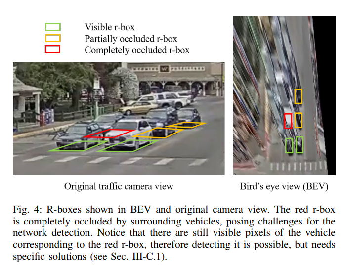
In bird’s eye view images, a large portion of the pixels of vehicles are outside of the r-boxes.
The IPM “stretches” the remote pixels, extending the remote vehicles to a long shape.
3.1. Tailed r-box regression
Propose a new regression target called tailed r-box to address the problem that r-boxes could be disjoint from the visible pixels of objects. It is constructed from the 3D bounding boxes in the original view.
The tail is defined as the line connecting the center of the bottom rectangle to that of the top rectangle of the 3D bounding box.
After warping to BEV, the tail extends from the r-box center through the stretched body of the vehicle, as shown below.
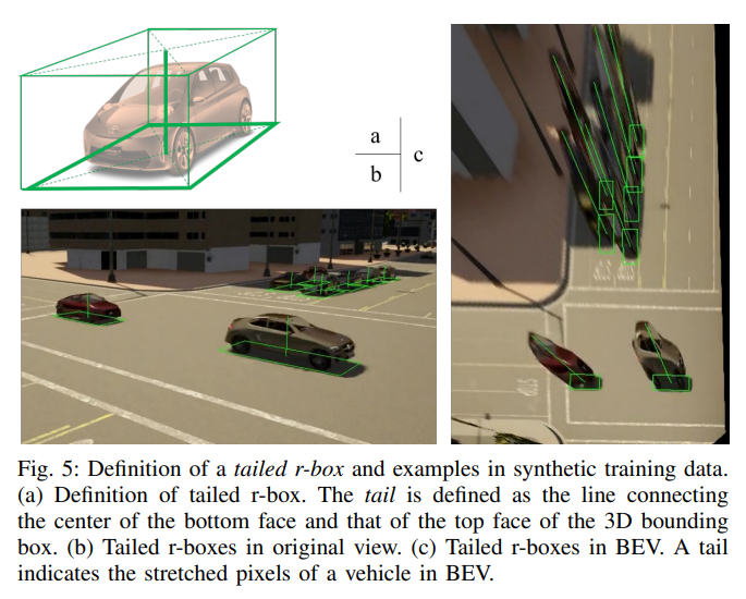
Note that while the definition of tails is in the original view images, the learning and inference of tails can be done in the BEV images . In BEV images, predicting tailed r-boxes corresponds to augmenting the prediction vector with two elements: $u_{tail}$, $v_{tail}$, representing the offset from the center of r-box to the end of tail in BEV. Anchors are not parameterized with tails.
=> By enforcing the network to predict the tail offset, the network is guided to learn that the stretched pixels far from the r-box are also part of the objects. Especially when the bottom part of a vehicle is occluded, the network could still detect it from the visible pixels at the top, drastically improving the recall rate. In comparison, directly regressing the projection of the 3D bounding boxes in BEV can achieve similar effect in guiding the network to leverage all pixels of a vehicle, but the projected location of the four top points is harder to determine in BEV, and creates unnecessary burden for the network.
3.2. Dual-view network architecture
In the dual-view network, there are two feature extractors with identical structures and non-shared parameters, taking BEV images and corresponding original view images as input respectively.
The feature maps of original images are then transformed to BEV through IPM and concatenated with the feature maps of the BEV images. The IPM of feature maps is similar to the IPM of raw images, with different homography matrices. The homography between the feature maps of original view and BEV can be calculated using Eq. 4.
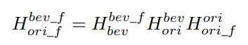
where $H^{bev_f}{bev}$ and $H^{ori}{ori_f}$ denotes the homography between the input image coordinates and the feature map coordinates, which are mainly determined by the pooling layers and convolution layers with strides.

With the dual-view architecture, pixels of a vehicle are spatially closer in the original view images than in the BEV images, making it easier to propagate information among the pixels. Then the intermediate feature warping stretches the information with IPM, propagating the consensus of nearby pixels of an object in the original view to pixels of further distances in BEV.
4. Data synthesis
Use CARLA-synthetic and Blender-synthetic

Experiments
- Quantitative result

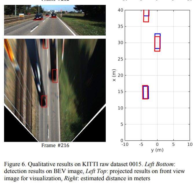
- Qualitative results

Conclusion
Proposed a new regression target called tailed rbox and a dual-view network architecture to address the distortion and occlusion problems which are common in warped BEV images.
provides a practical and generalizable solution to deploy 3D vehicle detection on already widely available traffic cameras. Many with unknown intrinsic/extrinsic calibration.
Deep Learning based Vehicle Position and Orientation Estimation via Inverse Perspective Mapping Image
(IV 2019)
Motivation
The information required in the autonomous driving system is the distance of the vehicle coordinate system. The detection result in the front view image cannot be used directly to predict the behavior of the detected vehicle. The bounding box of the front view image cannot distinguish whether the vehicle size is small or whether the vehicle looks small on far distance because the pixels of the front view image does not have distance information.
It is unfeasible to estimate the pose of the vehicle from the detection result on the front view image since the 2D bounding box covers the entire area of the vehicle even if the vehicle is oriented.
In order to make the distance measurement easier for the architecture, detecting the vehicle in the vehicle coordinate system can simplify the problem. For this purpose, the road of the front view image should be projected onto the bird’s eye view (BEV) image that is parallel and linear to the vehicle coordinate system. Although the vehicle appears distorted in the BEV image since the z-axis information is not preserved when projecting, the height of the road can be assumed to be zero if the camera motion is canceled. It can be supposed that all traffic participants are in contact with the ground in the road environment. Therefore, the distance can be estimated by detecting points where the vehicle is in contact with the road if the road plane of the front view image is well projected onto the BEV image.
Contribution
- Proposed a conceptually simple and effective method that estimates the position, size, and orientation of the vehicle in a meter unit on the BEV image. The main idea is that distance information can be restored by projecting the front image onto the BEV image if the road plane is parallel to the vehicle coordinate system.
Method
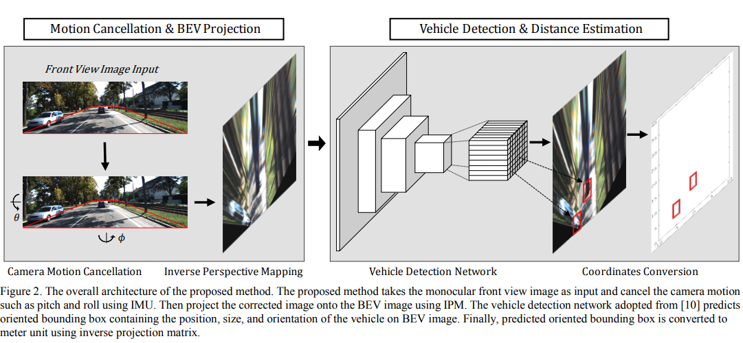
The proposed architecture takes front view image as input and cancels the camera pitch and roll motion using IMU. Then projects the corrected front view image onto the BEV image using the IPM. The one-stage object detector based vehicle detection network takes the BEV image and predicts the oriented bounding box composed of the position, size, and orientation. Finally, convert the predicted detection results of pixel units in the BEV image coordinate system into the distance of m units in the vehicle coordinate system.
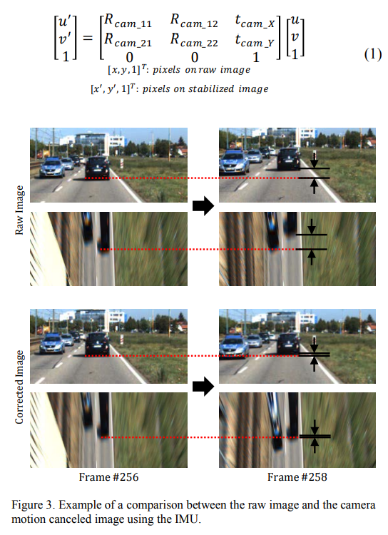
1. Motion Cancellation and BEV Projection
- Motion Cancellation using IMU: The motion cancellation is necessary to correct the motion of the ego vehicle caused by the wind disturbance or fluctuation of the road. The motion of the camera can be corrected by the extrinsic parameter of the camera and the rotation matrix of the IMU. The extrinsic parameter consists of the translation and rotation of the camera, and the rotation matrix consists of the pitch and roll angle.
- BEV projection:
Several assumptions are required to project the road surface in the front view image into the BEV image using IPM:
The surface where the ego vehicle and the surrounding vehicle drive is located must be a planar surface since IPM is a plane to plane transformation.
The mounting position of the camera must be stationary.
The vehicle to be detected must be attached to the ground plane because only the points on the ground have distance information.
2. Vehicle Detection and Distance Estimation
- Vehicle detection network:
- Distance estimation:
Since the detection network predicts the bottom box of the vehicle in contact with the road, the height of the detection result is zero. Therefore, the points on the road of the BEV image and vehicle coordinate system are defined by a one-to-one correspondence as

The matrix (4) is the product of the homography, motion cancellation matrix, intrinsic camera matrix, and transformation matrix of the camera. The point (x,y) on the BEV image coordinate system is converted into the point (X,Y) on the vehicle coordinate system using (4)
Experiments

Conclusion
- Fast
The Right (Angled) Perspective: Improving the Understanding of Road Scenes Using Boosted Inverse Perspective Mapping
(IV 2019)
Motivation
Cameras are one of the most popular sensing modalities in the field, due to their low cost as well as the availability of well-established image processing techniques.
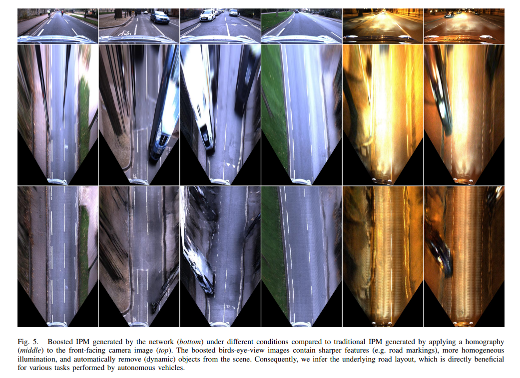
IPM problem: the geometric properties of objects in the distance are affected unnaturally by this non-homogeneous mapping.
Contribution
Introduce an Incremental Spatial Transformer GAN for generating boosted IPM in real time;
Explain how to create a dataset for training IPM methods on real-world images under different conditions; and
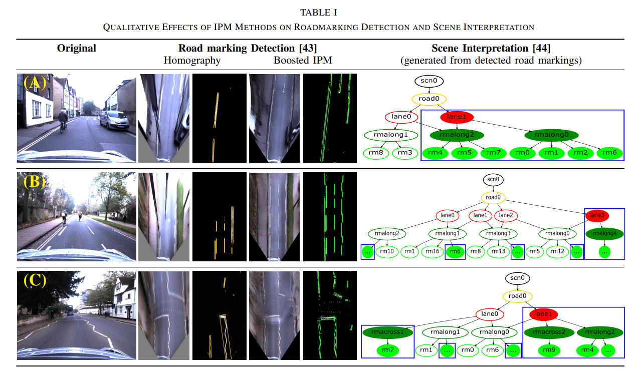
Demonstrate that our boosted IPM approach improves the detection of road markings as well as the semantic interpretation of road scenes in the presence of occlusions and/or extreme illumination.
Method
1. Boosted IPM using an incremental spatial transformer GAN
- Spatial ResNet Transformer
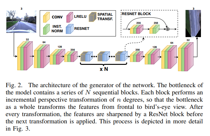
Since far-away real-world features are represented by a smaller pixel area as compared to identical close-by features, a direct consequence of applying a full perspective transformation to the input is increased unnatural blurring and stretching of the features at further distance. To counteract this effect, our model divides the full perspective transformation into a series of $N_{STRes}$ smaller incremental perspective transformations, each followed by a refinement of the transformed feature space using a ResNet block.
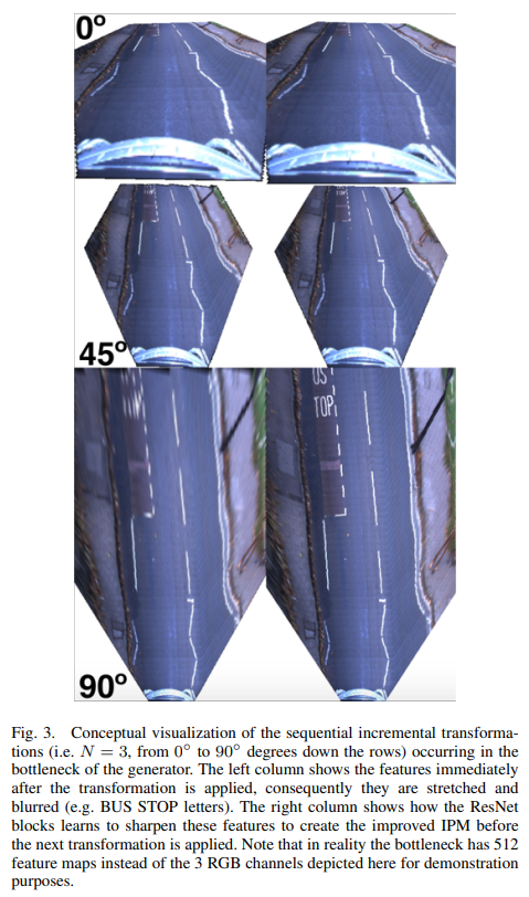
The intuition behind this is that the slight blurring that occurs as a result of each perspective transformation is restored by the ResNet block that follows it, as conceptually visualized in Fig. 3. To maintain the ability to train our model endto-end, we apply these incremental transforms using Spatial Transformers.
Intuitively, a Spatial Transformer is a mechanism, which can be integrated in a deep-learning pipeline, that warps an image using a parametrization (e.g. an affine or homography transformation matrix) conditioned on a specific input signal. Formally, each incremental spatial transformer is an end-toend differentiable sampler, represented in our case by two major components:
A convolutional network which receives an input I of size $H_I ∗ W_I ∗ C$, where $H_I$ , $W_I$ and $C$ represent the height, width, and number of channels of the input respectively, and outputs a parametrization $M_{loc}$ of a perspective transformation of size 3 ∗ 3, and;
A Grid Sampler which takes $I$ and $M_{loc}$ as inputs, creates a mapping matrix Mmap of size $H_O ∗W_O ∗ 2$, where $H_O$ and $W_O$ represent the height and width of the output $O$. Mmap maps homogeneous coordinates $[x, y, 1]^T$ to their new warped position given by $M_{loc} ∗ [x, y, 1]^T$. Finally, $M_{map}$ is used to construct $O$ in the following way: $O(x, y) = I(M_{map}(x, y, 1), M_{map}(x, y, 2))$.
In practice, it is non-trivial to train a spatial transformer (and even less trivial; a sequence of spatial transformers) on inputs with a large degree of self-similarity, such as road scenes. To stabilize the training procedure, for each incremental spatial transformer, we decompose $M_{loc} = M_{locref} ∗ M_{locpert}$ , where $M_{locref}$ is initialized with an approximate parametrization of the desired incremental homography, and $M_{locpert}$ is the actual output of the convolutional network and represents a learned perturbation or refinement of $M_{locref}$.
- Losses
With a generator $G$, $k^{th}$ scale discriminator $D_k$, and $L_{GAN}(G, D_k)$ being the traditional GAN loss defined over $k = 3$ scales, the final objective thus becomes:
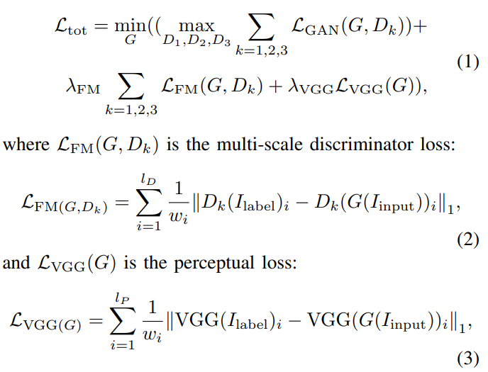
with $l_D$ denoting the number of discriminator layers used in the discriminator loss, $l_P$ denoting the number of layers from VGG16 that are utilized in the perceptual loss, and $I_{input}$ and $I_{label}$ being the input and label images, respectively. The weights $w_i = 2^{l−i}$ are used to scale the importance of each layer used in the loss.
2. Creating training data for boosted IPM
Experiments

Under certain conditions, the boosted IPM does not accurately depict all details of the bird’s-eye view of the scene. As we cannot enforce a pixel-wise loss during training, the shape of certain road markings is not accurately reflected (illustrated in Fig. 6). Improvement of the representation of these structural elements will be investigated in future work. Furthermore, the spatial transformer blocks assume that the road surface is more or less planar (and perpendicular to the z-axis of the vehicle). When this assumption is not satisfied, the network is unable to accurately reflect the top-down scene at further distance. This might be solved by providing/learning the rotation of the road surface with respect to the vehicle.
Conclusion
- No code
- Incremental Spatial Transformer GAN