
Spatial Transformer Networks
Convolutional Neural Networks (CNN) possess the inbuilt property of translation invariance. This enables them to correctly classify an image at test time, even when its constituent components are located at positions not seen during training. However, CNNs lack the inbuilt property of scale and rotation invariance: two of the most frequently encountered transformations in natural images. Since this property is not built in, it has to be learnt in a laborious way: during training, all relevant objects must be presented at different scales and rotations. This way the network learns a redundant set of features for each scale and each orientation, thus achieving the desired invariances. As a consequence, CNNs are usually very deep and require a lot of training data to gain high accuracies.
Spatial Transformer modules , introduced by Max Jaderberg et al., are a popular way to increase spatial invariance of a model against spatial transformations such as translation, scaling, rotation, cropping, as well as non-rigid deformations. They can be inserted into existing convolutional architectures: either immediately following the input or in deeper layers. They achieve spatial invariance by adaptively transforming their input to a canonical, expected pose, thus leading to a better classification performance. The word adaptive indicates, that for each sample an appropriate transformation is produced, conditional on the input itself. Spatial transformers networks can be trained end-to-end using standard backpropagation.
1. Forward and Reverse Mapping
1.1. Input Data
Spatial transformers are most commonly used on image data. A digital image consists of a finite number of tiny squares called pixels (pixel is short for picture element) organized into rows and columns. Each pixel value represents information, such as intensity or color.
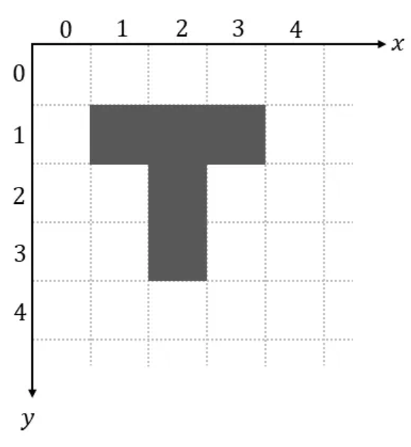
We use a coordinate system with the 𝑦-axis oriented downwards, as is common convention in computer vision.
The main characteristic of image data is the spatial relation between pixels. The spatial arrangement of pixels carries crucial information of the image content. Without the rest of the pixels, a single pixel has little meaning.
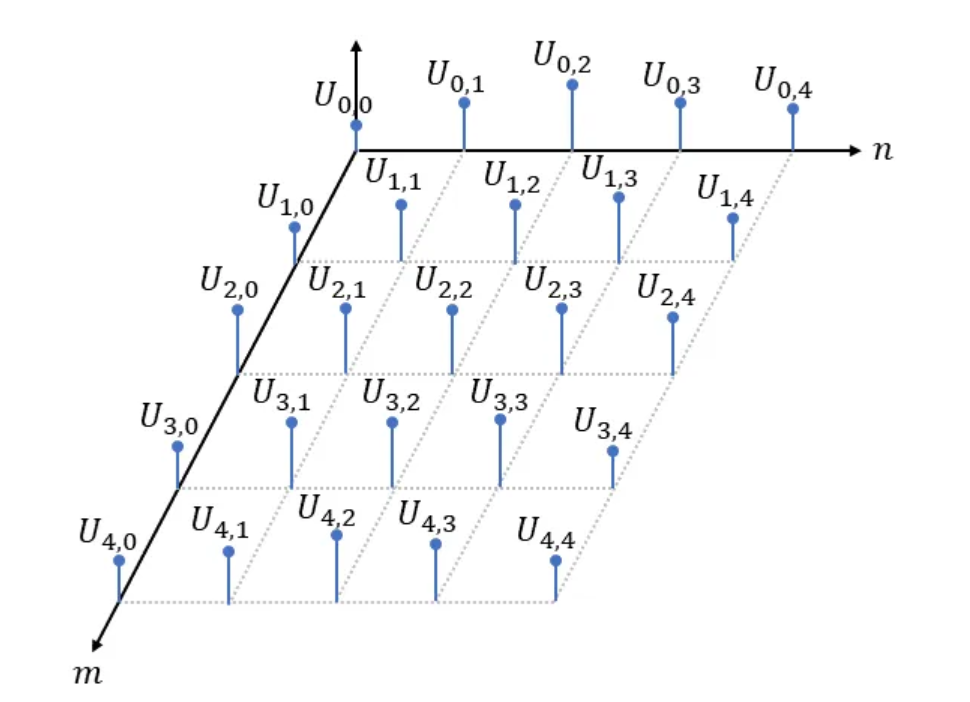
For reasons of clarity we will often use the “line plot” below to visualize image data in this tutorial. In this plot, spatial location is shown on the 𝑥-axis and 𝑦-axis with intensity values along the 𝑧-axis.
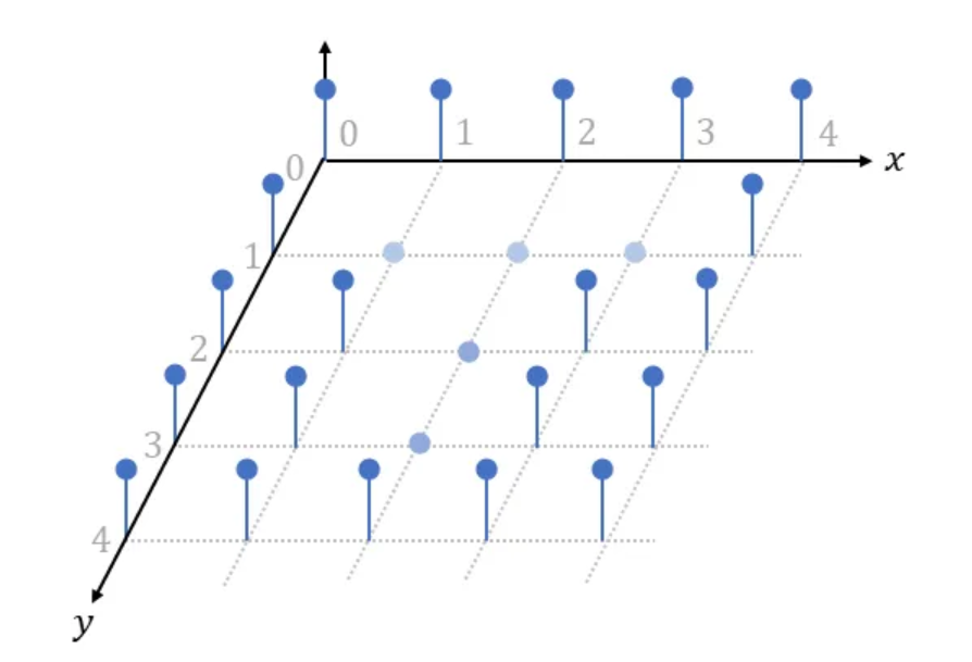
The line plot clearly illustrates the discrete nature of digital images, with pixel values only defined on the equally spaced grid and undefined outside.
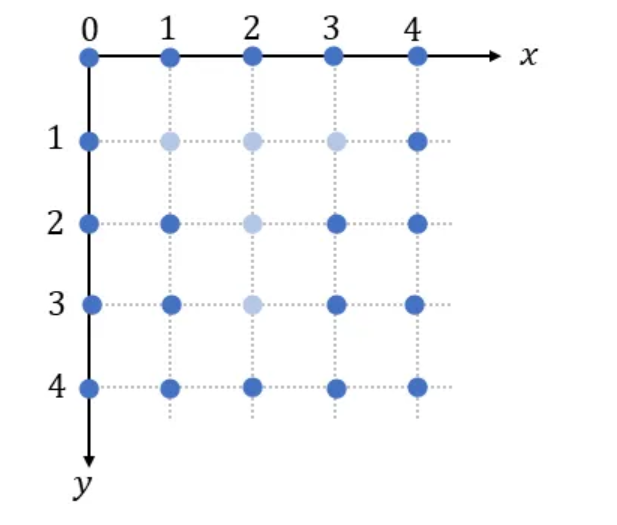
Whenever only spatial information is of importance, for example when we derive the gradients of the spatial transformer, we will use the following top-down view:
One thing to keep in mind: pixel values can be discrete or continuous. For example in a 8-bit grayscale image, each pixel has a discrete value ranging between 0 and 255, where 0 stands for black, and 255 stands for white. Feature maps, on the other hand, generated by convolutional layers have continuous pixel values.
1.2. Spatial Transformations
A spatial transformation moves each point (𝑦, 𝑥) of the input image to a new location (𝑣, 𝑢) in the output image, while preserving to some extent spatial relationships of pixels in neighborhoods:

The basic spatial transformations are scaling, rotation, translation and shear. Other important types of transformations are projections and mappings.
The forward transformation $𝑇{…}$ maps a location in input space to a location in output space:
\[(v, u) = T{(y, x)}\]The inverse transformation $𝑇^{-1}{…}$ maps a location in output space back to a location in input space:
\[(x, y) = T^{-1}\{(v, u)\}\]1.3. Forward Mapping
The most straight forward way to implement spatial transformations is to iterate over each pixel of the input image, compute its new location in the output image using $𝑇{…}$, and to copy the pixel value to the new location:

Most of the time the new locations (𝑣, 𝑢) will not fall on grid points in the output image (are not integer values). We solve this, by assigning the nearest integers to 𝑣 and 𝑢 and use these as output coordinates.
Forward mapping has two main disadvantages: overlaps and holes. As we see in the animation above, some output pixels receive more than one input image pixel, whereas other output pixels do not receive any input image pixels at all.
Due to the disadvantages of the forward mapping method, in practice a different technique, called reverse mapping, is used.
1.4 Reverse Mapping
Reverse mapping iterates over each pixel on the grid of the output image, uses the inverse transformation $𝑇^{-1}{…}$ to determine its corresponding position in the input image, samples the pixel value at this position, and uses that value as output pixel:

This method completely avoids problems with overlaps and holes. Reverse mapping is also the method used in spatial transformers.
As we have seen in the animation above, most of the time the determined positions in the input image (𝑦, 𝑥) don’t lie on the grid of the input image. In order to get an approximate value for the input image at these undefined non-integer positions, we must interpolate the pixel value. An interpolation technique called bilinear interpolation will be introduced in the next section.
1.5. Multiple Channels
So far, we have demonstrated the principles of forward mapping and reverse mapping on inputs with a single channel 𝐶 = 1, as encountered in e.g. grayscale images. However, most of the time inputs will have more than one channel 𝐶 > 1, such as RGB images which have three channels or feature maps in deep learning architectures which can have an arbitrary number of channels.
The extension is simple: for multi-channel inputs, the mapping is done identically for each channel of the input, so every channel is transformed in an identical way. This way we preserve spatial consistency between channels. Note, that spatial transformations do not change the number of channels 𝐶, which is same in input and output maps.
2. Bilinear Interpolation
2.1. Linear Interpolation
As a warm-up we will start with the simple one-dimensional case. Here we are dealing with a sequence of data points that lie on an equally spaced grid:

Since in this tutorial, we will mostly deal with image data, we can safely assume the space between two consecutive data points to be one without loss of generality.
Please note, that the discrete sequence in the diagram above is defined only for integer positions and undefined everywhere else. However, oftentimes we require values at non-integer positions, such as 2.7 in the above example. This is accomplished by interpolation techniques, which estimate the unknown data values from known data values. In the following, we will refer to undefined points, which we want to estimate using an interpolation technique, as sample points and denote them with letter 𝑥.
In linear interpolation we simply fit a straight line to only (!) two neighboring points of 𝑥 and then look up the desired value:

We find the neighboring points of 𝑥 by taking the floor and ceil operations. Remember: floor() rounds 𝑥 to the nearest integer below its value, whereas ceil() rounds it to the nearest integer above its value.

Since both neighboring points lie on the grid, we known their 𝑈 values (shown above to the right of the arrow). Furthermore, for two consecutive points on the grid we have that:

Next, we must fit the following straight line to the two neighboring points:

where 𝑚 is the slope and 𝑏 is the intersect. We obtain 𝑏 by plugging the left neighboring point into the equation:

The slope 𝑚 is obtained by plugging the right neighboring point into the equation:
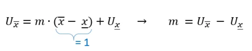
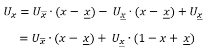
Our preliminary formula hence is:

To gain more intuition, let us expand the above product and rearrange:
Let us denote the distance from the sampling point 𝑥 to its right neighboring point as:

which we can also rewrite as:
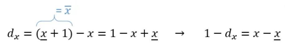
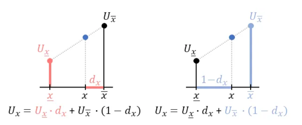
Thus, we arrive at our final formula:

See how linear interpolation can be interpreted in terms of the values of neighboring points weighted by opposite distances:
2.2. Bilinear Interpolation
Next, we will extend our foray to the two-dimensional case. Here we are dealing with a set of data points that lie on an equally spaced two-dimensional grid:
As in the 1-dimensional case, values at non-integer positions are undefined and must be estimated using interpolation techniques.
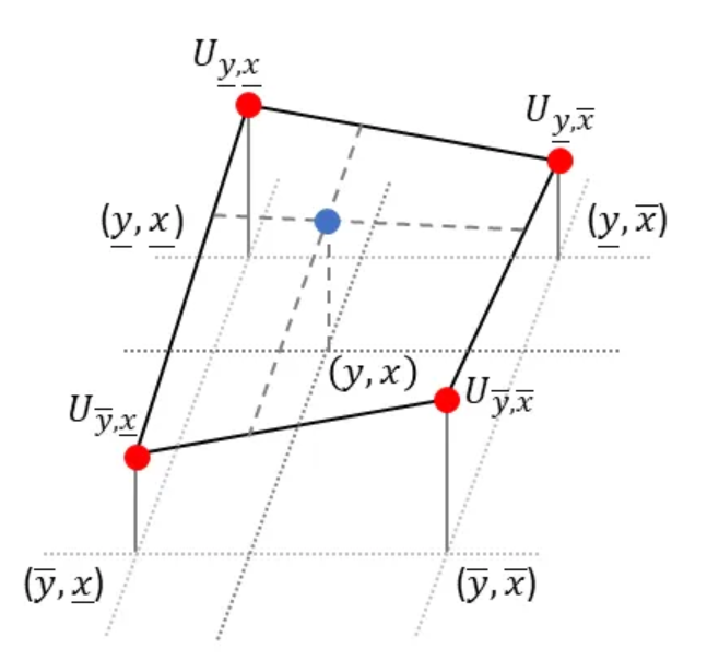
In bilinear interpolation we fit a plane to the closest four (!) neighboring points surrounding the sample point (𝑦, 𝑥) and then look up the desired value:
Luckily, to obtain the equation of the plane, we don’t need to solve a complicated system of linear equations, as done in the last section. Instead we will repeatedly apply linear interpolation (1-D) to two points each. We start with the upper two points and apply linear interpolation in horizontal direction. Next, we do the same for the lower two points. Finally, to obtain the desired value, we apply linear interpolation in vertical direction to the just obtained intermediate points, see animation below:
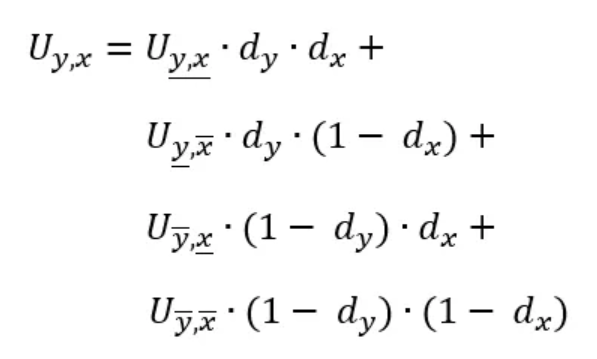
Linear interpolation in 𝑥-dimension:

Linear interpolation in 𝑦-dimension:

Combined, we get:
Due to symmetry, the order of the above two steps is irrelevant, i.e. carrying out the linear interpolation first in vertical direction and subsequently in horizontal direction, yields exactly the same formula.
Bilinear interpolation has also a nice geometric visualization: to obtain the value of the desired point (blue), we have to sum up the products of the value at each corner and the partial area diagonally opposite the corner:

There are two other important interpolation techniques called: nearest-neighbor interpolation and bicubic interpolation. The nearest-neighbor interpolation simply takes the nearest pixel to the sample point and copies it to the output location. Bicubic interpolation considers 16 neighbors of the sample point and fits a higher order polynomial to obtain the estimate.