Semantic segmentation tutorial [Part 1 Image Segmentaion]
Semantic segmentation: what is it?
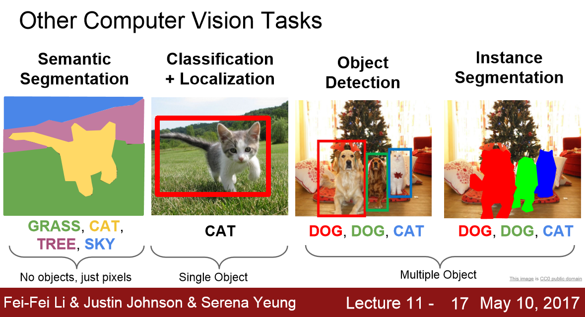
Semantic segmentation is the task of partitioning an image to coherent parts, and assigning a class label at each part. That is, per pixel classification of an image. This is an example of an image with it’s corresponding segmentation mask (i.e. the pixel labels). In this, green stands for trees, blue for buildings, yellow for cars and so on.
In this type of problems your training data will have sets of images and annotated masks, i.e. for each image, the mask will have exactly the same height and width as the image. Each pixel of the mask will contain some “class value”. The “class value” of the segmentation mask is usually represented with an integer, corresponding to a class, or an RGB (color) triplet.
What is important here, is to note that the format that the mask is given to you and the format of the mask expected from the loss function of the algorithm during training, are usually different things.
That is, you need to preprocess the data (masks) to bring them in an appropriate format for training. Anticipating an answer, assuming your classes are mutually exclusive (unless you are doing exotic embeddings, this will always be the case), the loss function during training expects masks into 1-hot encoding (the same goes for the predictions).
1-hot encoding is a way of representing categorical variables when they are mutually exclusive.
Methods and Techniques
Before the advent of deep learning, classical machine learning techniques like SVM, Random Forest, K-means Clustering were used to solve the problem of image segmentation. But as with most of the image related problem statements deep learning has worked comprehensively better than the existing techniques and has become a norm now when dealing with Semantic Segmentation. Let’s review the techniques which are being used to solve the problem.
Fully Convolutional Network
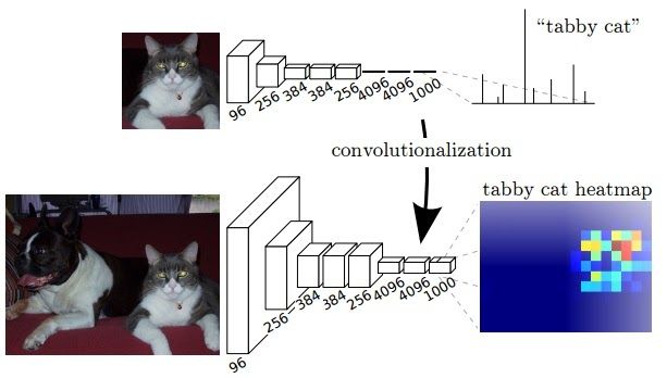
The general architecture of a CNN consists of few convolutional and pooling layers followed by few fully connected layers at the end. The paper of Fully Convolutional Network released in 2014 argues that the final fully connected layer can be thought of as doing a 1x1 convolution that cover the entire region.
Hence the final dense layers can be replaced by a convolution layer achieving the same result. But now the advantage of doing this is the size of input need not be fixed anymore. When involving dense layers the size of input is constrained and hence when a different sized input has to be provided it has to be resized. But by replacing a dense layer with convolution, this constraint doesn’t exist.
Also when a bigger size of image is provided as input the output produced will be a feature map and not just a class output like for a normal input sized image. Also the observed behavior of the final feature map represents the heatmap of the required class i.e the position of the object is highlighted in the feature map. Since the output of the feature map is a heatmap of the required object it is valid information for our use-case of segmentation.
Since the feature map obtained at the output layer is a down sampled due to the set of convolutions performed, we would want to up-sample it using an interpolation technique. Bilinear up sampling works but the paper proposes using learned up sampling with deconvolution which can even learn a non-linear up sampling.
The down sampling part of the network is called an encoder and the up sampling part is called a decoder. This is a pattern we will see in many architectures i.e reducing the size with encoder and then up sampling with decoder. In an ideal world we would not want to down sample using pooling and keep the same size throughout but that would lead to a huge amount of parameters and would be computationally infeasible.
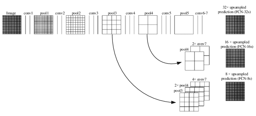
Although the output results obtained have been decent the output observed is rough and not smooth. The reason for this is loss of information at the final feature layer due to downsampling by 32 times using convolution layers. Now it becomes very difficult for the network to do 32x upsampling by using this little information. This architecture is called FCN-32
To address this issue, the paper proposed 2 other architectures FCN-16, FCN-8. In FCN-16 information from the previous pooling layer is used along with the final feature map and hence now the task of the network is to learn 16x up sampling which is better compared to FCN-32. FCN-8 tries to make it even better by including information from one more previous pooling layer.
U-Net
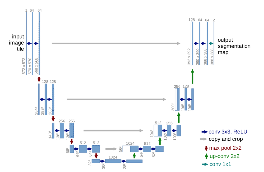
U-net builds on top of the fully convolutional network from above. It was built for medical purposes to find tumours in lungs or the brain. It also consists of an encoder which down-samples the input image to a feature map and the decoder which up samples the feature map to input image size using learned deconvolution layers.
The main contribution of the U-Net architecture is the shortcut connections. We saw above in FCN that since we down-sample an image as part of the encoder we lost a lot of information which can’t be easily recovered in the encoder part. FCN tries to address this by taking information from pooling layers before the final feature layer.
U-Net proposes a new approach to solve this information loss problem. It proposes to send information to every up sampling layer in decoder from the corresponding down sampling layer in the encoder as can be seen in the figure above thus capturing finer information whilst also keeping the computation low. Since the layers at the beginning of the encoder would have more information they would bolster the up sampling operation of decoder by providing fine details corresponding to the input images thus improving the results a lot. The paper also suggested use of a novel loss function which we will discuss below.
DeepLab
Deeplab from a group of researchers from Google have proposed a multitude of techniques to improve the existing results and get finer output at lower computational costs. The 3 main improvements suggested as part of the research are
1) Atrous convolutions 2) Atrous Spatial Pyramidal Pooling 3) Conditional Random Fields usage for improving final output Let’s discuss about all these
Atrous Convolution
One of the major problems with FCN approach is the excessive downsizing due to consecutive pooling operations. Due to series of pooling the input image is down sampled by 32x which is again up sampled to get the segmentation result. Downsampling by 32x results in a loss of information which is very crucial for getting fine output in a segmentation task. Also deconvolution to up sample by 32x is a computation and memory expensive operation since there are additional parameters involved in forming a learned up sampling.
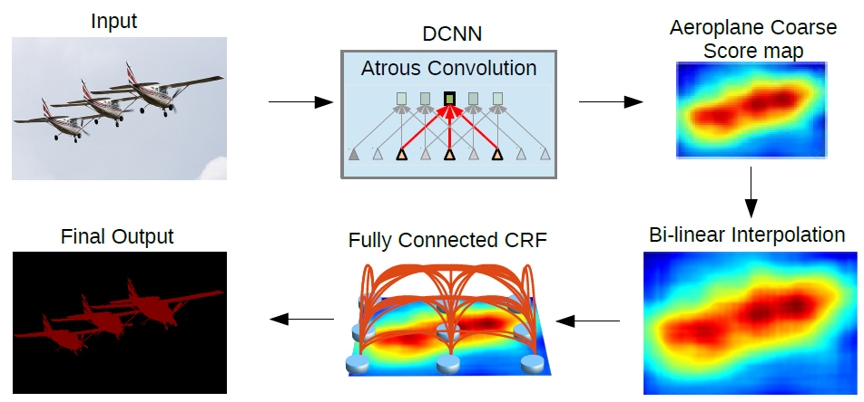
The paper proposes the usage of Atrous convolution or the hole convolution or dilated convolution which helps in getting an understanding of large context using the same number of parameters.
Dilated convolution works by increasing the size of the filter by appending zeros(called holes) to fill the gap between parameters. The number of holes/zeroes filled in between the filter parameters is called by a term dilation rate. When the rate is equal to 1 it is nothing but the normal convolution. When rate is equal to 2 one zero is inserted between every other parameter making the filter look like a 5x5 convolution. Now it has the capacity to get the context of 5x5 convolution while having 3x3 convolution parameters. Similarly for rate 3 the receptive field goes to 7x7.
In Deeplab last pooling layers are replaced to have stride 1 instead of 2 thereby keeping the down sampling rate to only 8x. Then a series of atrous convolutions are applied to capture the larger context. For training the output labelled mask is down sampled by 8x to compare each pixel. For inference, bilinear up sampling is used to produce output of the same size which gives decent enough results at lower computational/memory costs since bilinear up sampling doesn’t need any parameters as opposed to deconvolution for up sampling.
ASPP
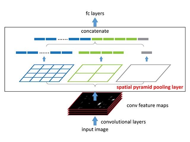
Spatial Pyramidal Pooling is a concept introduced in SPPNet to capture multi-scale information from a feature map. Before the introduction of SPP input images at different resolutions are supplied and the computed feature maps are used together to get the multi-scale information but this takes more computation and time. With Spatial Pyramidal Pooling multi-scale information can be captured with a single input image.
With the SPP module the network produces 3 outputs of dimensions 1x1(i.e GAP), 2x2 and 4x4. These values are concatenated by converting to a 1d vector thus capturing information at multiple scales. Another advantage of using SPP is input images of any size can be provided.
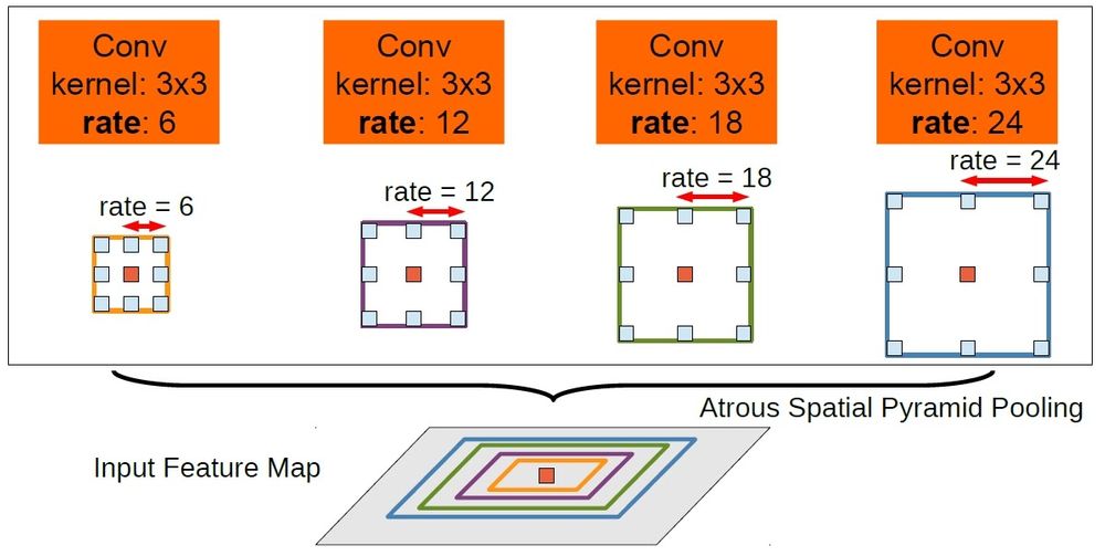
ASPP takes the concept of fusing information from different scales and applies it to Atrous convolutions. The input is convolved with different dilation rates and the outputs of these are fused together.
As can be seen the input is convolved with 3x3 filters of dilation rates 6, 12, 18 and 24 and the outputs are concatenated together since they are of same size. A 1x1 convolution output is also added to the fused output. To also provide the global information, the GAP output is also added to above after up sampling. The fused output of 3x3 varied dilated outputs, 1x1 and GAP output is passed through 1x1 convolution to get to the required number of channels.
Since the required image to be segmented can be of any size in the input the multi-scale information from ASPP helps in improving the results.
Improving output with CRF
Pooling is an operation which helps in reducing the number of parameters in a neural network but it also brings a property of invariance along with it. Invariance is the quality of a neural network being unaffected by slight translations in input. Due to this property obtained with pooling the segmentation output obtained by a neural network is coarse and the boundaries are not concretely defined.
To deal with this the paper proposes use of graphical model CRF. Conditional Random Field operates a post-processing step and tries to improve the results produced to define shaper boundaries. It works by classifying a pixel based not only on it’s label but also based on other pixel labels. As can be seen from the above figure the coarse boundary produced by the neural network gets more refined after passing through CRF.
Deeplab-v3 introduced batch normalization and suggested dilation rate multiplied by (1,2,4) inside each layer in a Resnet block. Also adding image level features to ASPP module which was discussed in the above discussion on ASPP was proposed as part of this paper
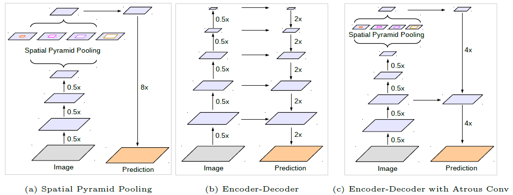
Deeplab-v3+ suggested to have a decoder instead of plain bilinear up sampling 16x. The decoder takes a hint from the decoder used by architectures like U-Net which take information from encoder layers to improve the results. The encoder output is up sampled 4x using bilinear up sampling and concatenated with the features from encoder which is again up sampled 4x after performing a 3x3 convolution. This approach yields better results than a direct 16x up sampling. Also modified Xception architecture is proposed to be used instead of Resnet as part of encoder and depthwise separable convolutions are now used on top of Atrous convolutions to reduce the number of computations.
Global Convolution Network
Semantic segmentation involves performing two tasks concurrently
i) Classification ii) Localization
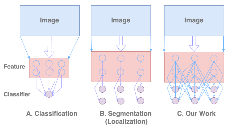
The classification networks are created to be invariant to translation and rotation thus giving no importance to location information whereas the localization involves getting accurate details w.r.t the location. Thus inherently these two tasks are contradictory. Most segmentation algorithms give more importance to localization i.e the second in the above figure and thus lose sight of global context. In this work the author proposes a way to give importance to classification task too while at the same time not losing the localization information
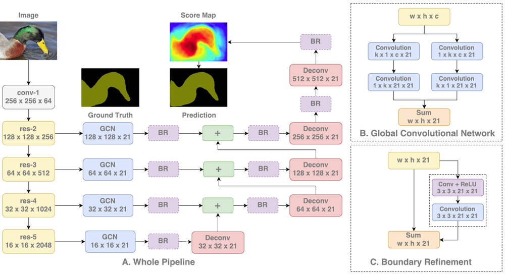
The author proposes to achieve this by using large kernels as part of the network thus enabling dense connections and hence more information. This is achieved with the help of a GCN block as can be seen in the above figure. GCN block can be thought of as a k x k convolution filter where k can be a number bigger than 3. To reduce the number of parameters a k x k filter is further split into 1 x k and k x 1, kx1 and 1xk blocks which are then summed up. Thus by increasing value k, larger context is captured.
In addition, the author proposes a Boundary Refinement block which is similar to a residual block seen in Resnet consisting of a shortcut connection and a residual connection which are summed up to get the result. It is observed that having a Boundary Refinement block resulted in improving the results at the boundary of segmentation.
Results showed that GCN block improved the classification accuracy of pixels closer to the center of object indicating the improvement caused due to capturing long range context whereas Boundary Refinement block helped in improving accuracy of pixels closer to boundary.
See More Than Once – KSAC for Semantic Segmentation
Deeplab family uses ASPP to have multiple receptive fields capture information using different atrous convolution rates. Although ASPP has been significantly useful in improving the segmentation of results there are some inherent problems caused due to the architecture. There is no information shared across the different parallel layers in ASPP thus affecting the generalization power of the kernels in each layer. Also since each layer caters to different sets of training samples(smaller objects to smaller atrous rate and bigger objects to bigger atrous rates), the amount of data for each parallel layer would be less thus affecting the overall generalizability. Also the number of parameters in the network increases linearly with the number of parameters and thus can lead to overfitting.
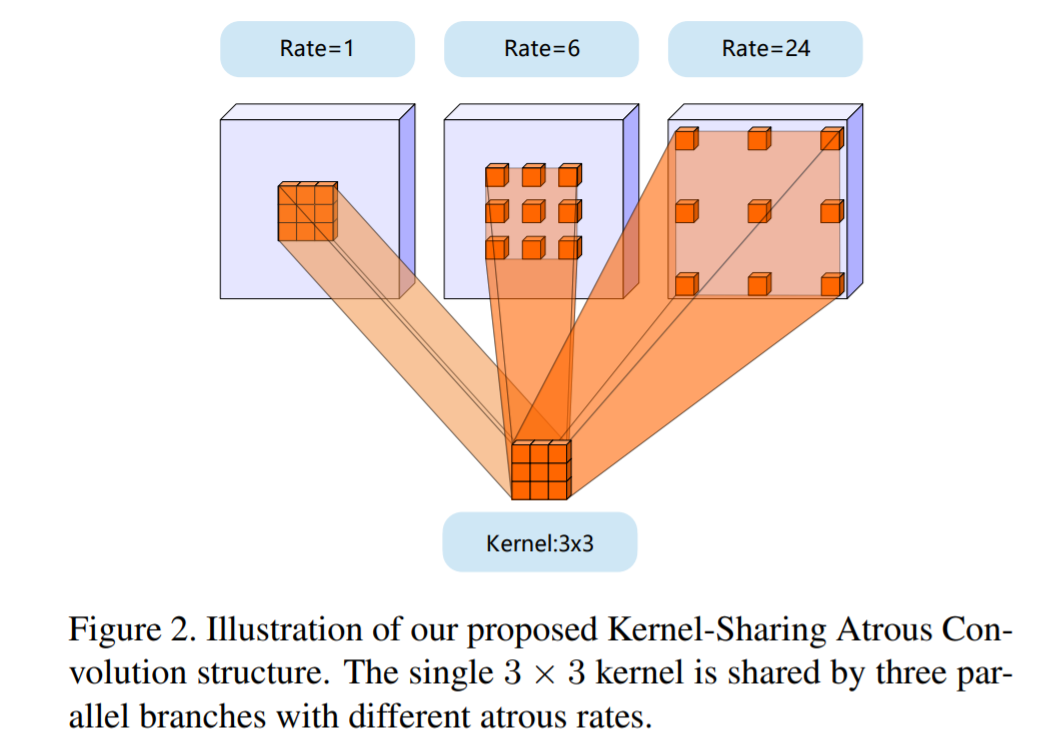
To handle all these issues the author proposes a novel network structure called Kernel-Sharing Atrous Convolution (KSAC). As can be seen in the above figure, instead of having a different kernel for each parallel layer is ASPP a single kernel is shared across thus improving the generalization capability of the network. By using KSAC instead of ASPP 62% of the parameters are saved when dilation rates of 6,12 and 18 are used.
Another advantage of using a KSAC structure is the number of parameters are independent of the number of dilation rates used. Thus we can add as many rates as possible without increasing the model size. ASPP gives best results with rates 6,12,18 but accuracy decreases with 6,12,18,24 indicating possible overfitting. But KSAC accuracy still improves considerably indicating the enhanced generalization capability.
This kernel sharing technique can also be seen as an augmentation in the feature space since the same kernel is applied over multiple rates. Similar to how input augmentation gives better results, feature augmentation performed in the network should help improve the representation capability of the network.
